一、课题简介

可以直接当机器学习课设。

股票涨跌预测，选用了一个具有3556行数据，25个特征的真实csv数据集，我将会为此数据集在jupyter 上使用机器学习相关Python库进行数据集的读取分析，根据具体的情况进行数据预处理，步骤包含缺失值重复值检测，选取与目标涨跌%%相关的特征重新定义新数据集，标准化，pca主成分降维，拆分训练集数据和测试集数据。

我根据此数据集的复杂度选取了随机森林机器学习模型和支持向量机模型进行建模，首先进行交叉验证与网格搜索结合和网格搜索不断的训练评估，选取它们的最优参数，然后得出它们在训练集和测试集评分，用模型预测测试集，得出模型均方误差，最后绘制出预测值和实际值的对比图，加上标题和图例。

二、数据准备

首先导入pandas和numpy,再从sklearn里面导出数据拆分模块和标准化模块。还有均方误差评估模块和matplotlib画图模块,添加上能够正常显示中文的两行代码

#导入模块
import pandas as pd
import numpy as np
from sklearn.model_selection import train_test_split
from sklearn.preprocessing import StandardScaler
from sklearn.cluster import KMeans  
from sklearn.metrics import silhouette_score  
from sklearn.metrics import mean_squared_error

from matplotlib import pyplot as plt 
plt.rcParams['font.sans-serif']=['SimHei'] #用来正常显示中文标签
plt.rcParams['axes.unicode_minus']=False

数据收集：

用pandas里面的read_csv来导入数据集。指定格式为gb k能够正常显示中文。data.dropna(inplace=True),将数据集中包含缺失值的行进行删除，并替代原数据集，然后显示数据集的前五行。

# 数据读取
data = pd.read_csv(
   "C:\\Users\\nhean\\Desktop\\股票数据.csv",
     encoding='gbk')
data.dropna(inplace=True)
data.head()

	代码	名称	涨幅%%	现价	涨跌	买价	卖价	总量	现量	涨速%%	...	总金额	量比	振幅%%	均价	内盘	外盘	内外比	买量	卖量	开盘金额
0	1	平安银行	2.89	11.05	0.31	11.05	11.06	2110243	17125	0.00	...	2331358208	1.89	4.56	11.05	973030	1137212	0.86	3547	9651	4028900
1	2	万 科Ａ	-0.61	24.30	-0.15	24.30	24.31	683236	8615	0.04	...	1671576704	0.90	3.89	24.47	339287	343949	0.99	563	594	2508800
2	4	国农科技	0.38	15.90	0.06	15.90	15.91	2243	50	0.19	...	3569043	0.33	2.46	15.91	1042	1201	0.87	271	37	1600
3	5	世纪星源	-0.34	2.94	-0.01	2.93	2.94	57901	1275	0.34	...	17088052	0.86	2.71	2.95	36647	21253	1.72	1390	926	3300
4	6	深振业Ａ	0.88	5.70	0.05	5.70	5.71	413030	6352	0.18	...	236936288	0.71	5.13	5.74	198243	214787	0.92	1193	1344	847100

5 rows × 26 columns

打印详情可以看到有多少行数据集，有多少个特征，和有没有缺失值

#打印详情
data.info()

<class 'pandas.core.frame.DataFrame'>
RangeIndex: 3556 entries, 0 to 3555
Data columns (total 26 columns):
 #   Column  Non-Null Count  Dtype  
---  ------  --------------  -----  
 0   代码      3556 non-null   int64  
 1   名称      3556 non-null   object 
 2   涨幅%%    3556 non-null   float64
 3   现价      3556 non-null   float64
 4   涨跌      3556 non-null   float64
 5   买价      3556 non-null   float64
 6   卖价      3556 non-null   float64
 7   总量      3556 non-null   int64  
 8   现量      3556 non-null   int64  
 9   涨速%%    3556 non-null   float64
 10  换手%%    3556 non-null   float64
 11  今开      3556 non-null   float64
 12  最高      3556 non-null   float64
 13  最低      3556 non-null   float64
 14  昨收      3556 non-null   float64
 15  市盈(动)   3556 non-null   float64
 16  总金额     3556 non-null   int64  
 17  量比      3556 non-null   float64
 18  振幅%%    3556 non-null   float64
 19  均价      3556 non-null   float64
 20  内盘      3556 non-null   int64  
 21  外盘      3556 non-null   int64  
 22  内外比     3556 non-null   float64
 23  买量      3556 non-null   int64  
 24  卖量      3556 non-null   int64  
 25  开盘金额    3556 non-null   int64  
dtypes: float64(16), int64(9), object(1)
memory usage: 722.4+ KB
检测重复值显示为零不用进行处理
#重复值检测，无重复
data.duplicated().sum()
0

用 corr() 方法计算每对属性之间的皮尔逊相关系数。相关系数范围 [-1, 1] ，越接近 1 表示有越强的正相关，越接近 -1 表示有越强的负相关。具体看每个属性与房价中位数的相关性。，为负数的可以删去

new_data1= data.drop(['代码', '名称'], axis=1)
#用 corr() 方法计算每对属性之间的皮尔逊相关系数。相关系数范围 [-1, 1] ，越接近 1 表示有越强的正相关，越接近 -1 表示有越强的负相关。
cor=new_data1.corr()
#具体看每个属性与房价中位数的相关性。
cor['涨幅%%'].sort_values(ascending=False)
幅%%     1.000000
涨跌       0.699442
振幅%%     0.364492
量比       0.263082
买量       0.231196
换手%%     0.104710
涨速%%     0.097853
买价       0.064713
外盘       0.062571
最高       0.057390
最低       0.052498
现价       0.050793
今开       0.048643
均价       0.047879
昨收       0.037048
总金额      0.035917
总量       0.033600
卖价       0.031857
市盈(动)    0.025833
内盘      -0.003812
开盘金额    -0.020553
现量      -0.028021
内外比     -0.085523
卖量      -0.171343
Name: 涨幅%%, dtype: float64

用data.drop删除与分类数无关的特征与我们要预测的涨幅%%特征，axis=1指定删除列 储存在new_data中显示头部5行

new_data = data.drop(['代码', '名称','涨幅%%','内盘','现量','卖量','内外比','开盘金额','卖量'], axis=1)
new_data.head()

	现价	涨跌	买价	卖价	总量	涨速%%	换手%%	今开	最高	最低	昨收	市盈(动)	总金额	量比	振幅%%	均价	外盘	买量
0	11.05	0.31	11.05	11.06	2110243	0.00	1.23	10.78	11.27	10.78	10.74	7.09	2331358208	1.89	4.56	11.05	1137212	3547
1	24.30	-0.15	24.30	24.31	683236	0.04	0.70	24.50	24.90	23.95	24.45	14.70	1671576704	0.90	3.89	24.47	343949	563
2	15.90	0.06	15.90	15.91	2243	0.19	0.27	15.80	16.12	15.73	15.84	336.53	3569043	0.33	2.46	15.91	1201	271
3	2.94	-0.01	2.93	2.94	57901	0.34	0.61	2.96	2.99	2.91	2.95	191.01	17088052	0.86	2.71	2.95	21253	1390
4	5.70	0.05	5.70	5.71	413030	0.18	3.06	5.61	5.88	5.59	5.65	9.25	236936288	0.71	5.13	5.74	214787	1193

拆分数据集：

我们选择new_data作为特征，'涨幅%%'作为标签，用train_test_split，按测试集占百分之二十拆分，随机种子为42号，这样重新加载不会改变拆分结果

# 特征选择
# 假设我们选择以下列作为特征，'涨幅%%'作为标签
features = new_data
labels = data['涨幅%%']
# 拆分数据集为训练集测试集
# test_size: 测试集的比例
# random_state: 随机种子，确保结果可复现
X_train, X_test, y_train, y_test = train_test_split(features, labels, test_size=0.2, random_state=42)
# 查看分割后的数据集大小
print(X_train.shape, X_test.shape)

(2844, 18) (712, 18)

三、数据预处理

标准化：

使用StandardScaler()进行标准化，对训练集进行训练和数据转换，对测试集进行数据转换，定义转换对象，无报错成功转换

scaler = StandardScaler()
X_train_scaled = scaler.fit_transform(X_train)
X_test_scaled = scaler.transform(X_test)

PCA降维:

导入pca，设置主成分为2，对标准化后的训练集进行拟合，对标准化后的训练集数据进行降维，对标准化后的测试集数据进行降维，最后打印维度，降维成功

#导入pca
from sklearn.decomposition import PCA
#设置主成分为2
pca=PCA(n_components=2)
#对标准化后的训练集进行拟合
pca.fit(X_train_scaled)
#对标准化后的训练集数据进行降维
X_train_pca=pca.transform(X_train_scaled)
#对标准化后的测试集数据进行降维
X_test_pca=pca.transform(X_test_scaled)
print('降维后训练集的维度为：',X_train_pca.shape)
print('降维后测试集的维度为：',X_test_pca.shape)

降维后训练集的维度为： (2844, 2)
降维后测试集的维度为： (712, 2)

四、建模与评估

模型选取：

鉴于这是一个拥有多个特征和三千多条数据的股票数据集，我选择的第一个模型是支持向量机它在高维数据（股票数据有多种特征）中有优势，能有效处理非线性关系，找到合适的决策边界，对股票价格走势等复杂关系进行分类或预测，第二个模型是随机森林，它可以处理大量的特征，并且能够评估特征的重要性，在复杂的股票数据中筛选出对股价波动等关键因素有重要影响的特征，还能有效减少过拟合，提高模型的泛化能力。

模型1随机森林：

使用到了交叉验证与网格搜索结合的方法，从sklearn导入cross_val_score和随机森林模块，定义一个最高分best_score，随机森林有两个参数分别为n_estimator和random_state,它们分别为n和r，遍历这2个列表，内的参数是不断调优后得到的，原理是不断地训练验证打印最高分存在best_score里面，最后输出它的最优参数

#交叉验证评估与网格搜索结合
from sklearn.model_selection import cross_val_score
from sklearn.ensemble import RandomForestRegressor
best_score=0
for n in [340,344,350]:
    for r in [1,2,5]:
        model1= RandomForestRegressor(n_estimators=n, random_state=r)
        scores=cross_val_score(model1,X_train_scaled,y_train,cv=5)
        score=np.mean(scores)
        if score>best_score:
            best_score=score
            best_params={'n_estimators':n,'random_state':r}
print('交叉验证的最高分:{:.3f}'.format(best_score))
print('最优参数：{}'.format(best_params))

交叉验证的最高分:0.950
最优参数：{'n_estimators': 350, 'random_state': 2}

根据上面的选取参数进行最终建模，打印训练集和测试集评分，用测试集进行模型预测计算出均方误差并打印

# 根据交叉验证评估得出的最优参数建模
model1 = RandomForestRegressor(n_estimators=350, random_state=2)
model1.fit(X_train_scaled, y_train)
#评估模型
print('训练集评分：{:.2f}'.format(model1.score(X_train_scaled,y_train)))
print('测试集评分：{:.2f}'.format(model1.score(X_test_scaled ,y_test)))
# 模型预测
predictions = model1.predict(X_test_scaled)
 
# 计算均方误差
svr_mse = mean_squared_error(y_test, predictions)
 
print(f"模型的均方误差: {svr_mse:.2f}")

训练集评分：0.99
测试集评分：0.93
模型的均方误差: 0.30

模型2支持向量机：

用网格搜索查找最优参数，支持向量机模型有两个参数，gamma和C，定义列表遍历他们不断地用svm训练打印得分评估，储存在best_score里面，最终打印最高得分和他的参数

#网格搜索找最优参数
from sklearn.svm import SVR
best_score=0
for gamma in [0.001,0.01,0.1,1,10]:
    for C in [90,100,120]:
        svm=SVR(gamma=gamma,C=C)
        svm.fit(X_train_scaled,y_train)
        score=svm.score(X_test_scaled,y_test)
        if score>best_score:
            best_score=score
            best_params={'gamma':gamma,'C':C}
print('模型最高分:{:.3f}'.format(best_score))
print('最优参数：{}'.format(best_params))

模型最高分:0.946
最优参数：{'gamma': 0.01, 'C': 120}

根据上面的选取参数进行最终建模，打印训练集和测试集评分，用测试集进行模型预测计算出均方误差并打印

from sklearn.svm import SVR
# 用最优参数训练支持向量回归模型
svr_model = SVR(kernel='rbf', C=120, gamma=0.01)
svr_model.fit(X_train_scaled, y_train)
 
# 模型预测
svr_predictions = svr_model.predict(X_test_scaled)
 
# 计算均方误差
svr_mse = mean_squared_error(y_test, svr_predictions)
 
print(f"SVR模型的均方误差: {svr_mse:.2f}")
#评估模型
print('训练集评分：{:.2f}'.format(svr_model.score(X_train_scaled,y_train)))
print('测试集评分：{:.2f}'.format(svr_model.score(X_test_scaled,y_test)))

SVR模型的均方误差: 0.22
训练集评分：0.97
测试集评分：0.95

五、结果分析与展示

模型分析图示：

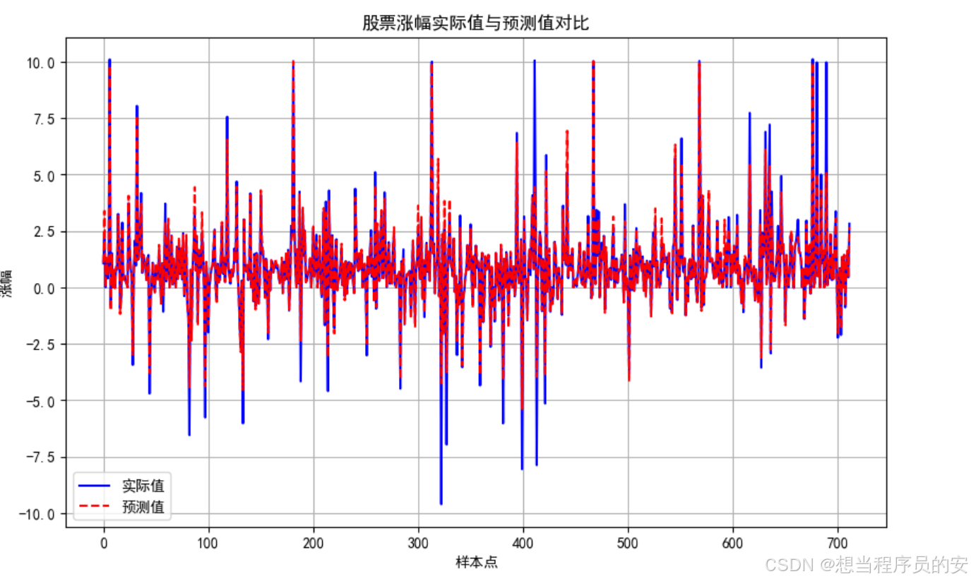
模型1：

plt.figure(figsize=(10, 6)) 定义图的大小，plt.plot(y_test.values, label='实际值', color='blue')用测试集的值，画出实际值曲线，颜色为蓝色，plt.plot(predictions, label='预测值', linestyle='--', color='red')用预测的结果，画出预测值曲线，线型为虚线，颜色为红色方便对比观察。

# 绘制实际值与预测值对比图
plt.figure(figsize=(10, 6))
plt.plot(y_test.values, label='实际值', color='blue')
plt.plot(predictions, label='预测值', linestyle='--', color='red')
plt.xlabel('样本点')
plt.ylabel('涨幅')
plt.title('股票涨幅实际值与预测值对比')
plt.legend()
plt.grid()
plt.show()

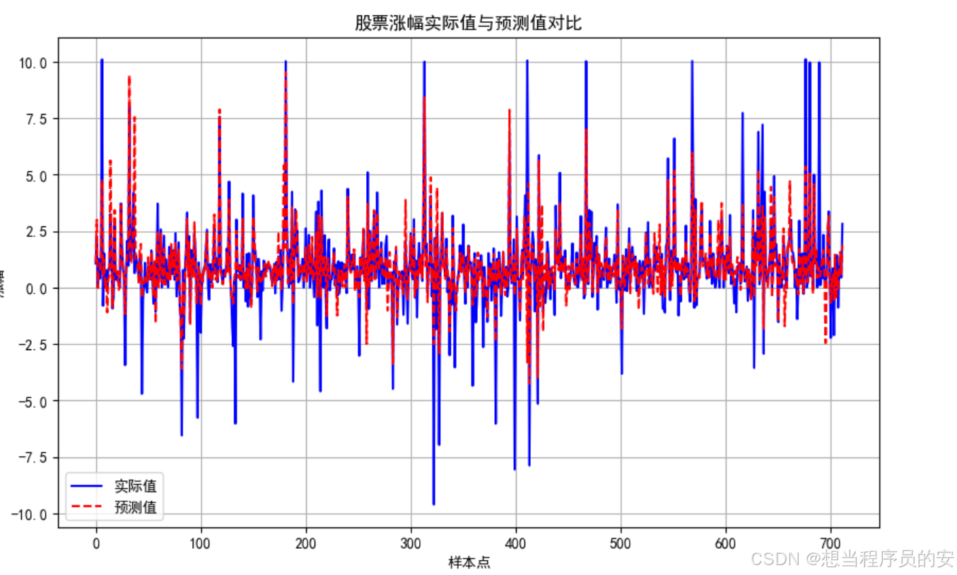
模型2：

代码与上面一样，改变了预测值画图的这一行代码，plt.plot(svr_predictions, label='SVR预测值', linestyle='--', color='red')，绘出svr_predictions的数值曲线

# 绘制实际值与预测值对比图
plt.figure(figsize=(10, 6))
plt.plot(y_test.values, label='实际值', color='blue')
plt.plot(svr_predictions, label='SVR预测值', linestyle='--', color='red')
plt.xlabel('样本点')
plt.ylabel('收盘价')
plt.title('股票收盘价实际值与预测值对比')
plt.legend()
plt.grid()
plt.show()