Python数据处理与分析小项目-分析员工过早离职原因
通过描述性分析、相关性分析、变量之间的对比分析来解析影响公司员工离职的因素。以及公司应该思考和解决的问题。
项目介绍
- 背景说明
本篇通过描述性分析、相关性分析、变量之间的对比分析来解析影响公司员工离职的因素。以及公司应该思考和解决的问题。
人力资源分析数据集汇聚了对大量员工的信息数据统计,包括企业因素(如部门)、员工行为相关因素(如参与过项目数、每月工作时长、薪资水平等)、以及工作相关因素(如绩效评估、工伤事故)
- 数据说明
文件HR_comma_sep.csv中包含10个字段,具体信息如下:
| No | 属性 | 数据类型 | 字段描述 |
|---|---|---|---|
| 1 | satisfaction_level | Float | 员工满意程度:0-不满意,1-满意 |
| 2 | last_evaluation | Float | 国家 |
| 3 | number_project | Integer | 在职期间完成的项目数量 |
| 4 | average_montly_hours | Integer | 每月平均工作时长(hr) |
| 5 | time_spend_company | Integer 工龄(年) | |
| 6 | work_accident | Integer | 是否有工伤:0-没有,1-有 |
| 7 | left | Integer | 是否离职:0-在职,1-离职 |
| 8 | promotion_last_5years | Integer | 过去5年是否有升职:0-没有,1-有 |
| 9 | sales | String | 工作部门 |
| 10 | salary | String | 工资的相对等级 |
- 数据来源
https://www.kaggle.com/mizanhadi/hr-employee-data-visualisation/data?select=HR_comma_sep.csv
百度云下载链接:
链接:https://pan.baidu.com/s/1G3uT2Bs7MUnjrFmh4vB_Xg
提取码:abcd
安装相关包
!pip install plotly==2.7.0 -i https://pypi.tuna.tsinghua.edu.cn/simple --trusted-host pypi.tuna.tsinghua.edu.cn
!pip install colorlover -i https://pypi.tuna.tsinghua.edu.cn/simple --trusted-host pypi.tuna.tsinghua.edu.cn
导入相关包
import pandas as pd
import numpy as np

from plotly import __version__
print (__version__)

from plotly.offline import init_notebook_mode, iplot
init_notebook_mode(connected=True)
from plotly.graph_objs import *
import colorlover as cl

import matplotlib.pyplot as plt
import seaborn as sns
colors = ['#e43620', '#f16d30','#d99a6c','#fed976', '#b3cb95', '#41bfb3','#229bac', '#256894']
2.7.0
1.数据检查与理解
data = pd.read_csv('./HR_comma_sep.csv')
data.head()
| satisfaction_level | last_evaluation | number_project | average_montly_hours | time_spend_company | Work_accident | left | promotion_last_5years | sales | salary | |
|---|---|---|---|---|---|---|---|---|---|---|
| 0 | 0.38 | 0.53 | 2 | 157 | 3 | 0 | 1 | 0 | sales | low |
| 1 | 0.80 | 0.86 | 5 | 262 | 6 | 0 | 1 | 0 | sales | medium |
| 2 | 0.11 | 0.88 | 7 | 272 | 4 | 0 | 1 | 0 | sales | medium |
| 3 | 0.72 | 0.87 | 5 | 223 | 5 | 0 | 1 | 0 | sales | low |
| 4 | 0.37 | 0.52 | 2 | 159 | 3 | 0 | 1 | 0 | sales | low |
print("共有",data.shape[0],"条员工记录,",data.shape[1],"个员工特征。")
共有 14999 条员工记录, 10 个员工特征。
1.1. 检查是否存在缺失值
data.isnull().sum()
satisfaction_level       0
last_evaluation          0
number_project           0
average_montly_hours     0
time_spend_company       0
Work_accident            0
left                     0
promotion_last_5years    0
sales                    0
salary                   0
dtype: int64
1.2. 适当的改名来更直观的理解和获取特征列
df = data.rename(columns = {"sales":"department","promotion_last_5years":"promotion","Work_accident":"work_accident"})
df.columns
Index(['satisfaction_level', 'last_evaluation', 'number_project',
       'average_montly_hours', 'time_spend_company', 'work_accident', 'left',
       'promotion', 'department', 'salary'],
      dtype='object')
1.3. 查看数据的信息
df.info()
<class 'pandas.core.frame.DataFrame'>
RangeIndex: 14999 entries, 0 to 14998
Data columns (total 10 columns):
 #   Column                Non-Null Count  Dtype
---  ------                --------------  -----
 0   satisfaction_level    14999 non-null  float64
 1   last_evaluation       14999 non-null  float64
 2   number_project        14999 non-null  int64
 3   average_montly_hours  14999 non-null  int64
 4   time_spend_company    14999 non-null  int64
 5   work_accident         14999 non-null  int64
 6   left                  14999 non-null  int64
 7   promotion             14999 non-null  int64
 8   department            14999 non-null  object
 9   salary                14999 non-null  object
dtypes: float64(2), int64(6), object(2)
memory usage: 1.1+ MB
1.4. 展示所有类型特征的信息
df.describe(include=['O'])
| department | salary | |
|---|---|---|
| count | 14999 | 14999 |
| unique | 10 | 3 |
| top | sales | low |
| freq | 4140 | 7316 |
1.5. 类别数字化
- 先设置
salary与department列为Category的数据类型 - 保存类别与对应数值的映射字典
- 针对
salary和department这两个Object类型的类别特征,将其进行类别数字化。
# 1. 先设置`salary`与`department`列为**Category**的数据类型
df['department'] = df['department'].astype('category')#, categories=cat.categories)
df['salary'] = df['salary'].astype('category')#, categories=cat.categories)
df.info()
<class 'pandas.core.frame.DataFrame'>
RangeIndex: 14999 entries, 0 to 14998
Data columns (total 10 columns):
 #   Column                Non-Null Count  Dtype
---  ------                --------------  -----
 0   satisfaction_level    14999 non-null  float64
 1   last_evaluation       14999 non-null  float64
 2   number_project        14999 non-null  int64
 3   average_montly_hours  14999 non-null  int64
 4   time_spend_company    14999 non-null  int64
 5   work_accident         14999 non-null  int64
 6   left                  14999 non-null  int64
 7   promotion             14999 non-null  int64
 8   department            14999 non-null  category
 9   salary                14999 non-null  category
dtypes: category(2), float64(2), int64(6)
memory usage: 967.4 KB
# 保存类别
# department_categories = pd.Categorical(df['department']).categories
# salary_categories = pd.Categorical(df['salary']).categories
# 2. 保存类别与对应数值的映射字典
salary_dict = dict(enumerate(df['salary'].cat.categories))
department_dict = dict(enumerate(df['department'].cat.categories))
salary_dict,department_dict
({0: 'high', 1: 'low', 2: 'medium'},
 {0: 'IT',
  1: 'RandD',
  2: 'accounting',
  3: 'hr',
  4: 'management',
  5: 'marketing',
  6: 'product_mng',
  7: 'sales',
  8: 'support',
  9: 'technical'})
# 3. 针对`salary`和`department`这两个`Object`类型的类别特征,将其进行类别数字化。
for feature in df.columns:
    if str(df[feature].dtype) == 'category':
        df[feature] = df[feature].cat.codes
        # df[feature] = pd.Categorical(df[feature]).codes
        df[feature] = df[feature].astype("int64") # 设置数据类型为int64
df.head()
| satisfaction_level | last_evaluation | number_project | average_montly_hours | time_spend_company | work_accident | left | promotion | department | salary | |
|---|---|---|---|---|---|---|---|---|---|---|
| 0 | 0.38 | 0.53 | 2 | 157 | 3 | 0 | 1 | 0 | 7 | 1 |
| 1 | 0.80 | 0.86 | 5 | 262 | 6 | 0 | 1 | 0 | 7 | 2 |
| 2 | 0.11 | 0.88 | 7 | 272 | 4 | 0 | 1 | 0 | 7 | 2 |
| 3 | 0.72 | 0.87 | 5 | 223 | 5 | 0 | 1 | 0 | 7 | 1 |
| 4 | 0.37 | 0.52 | 2 | 159 | 3 | 0 | 1 | 0 | 7 | 1 |
1.6. 改变columns的顺序
1.先设置columns的顺序
- 将left列放置于最后一列以便直观地查看
2.根据排好的列表顺序应用于dataframe上
cols = df.columns
cols = list(cols[:6]) + list(cols[7:]) + [cols[6]]
print('Reordered Columns:',cols)
Reordered Columns: ['satisfaction_level', 'last_evaluation', 'number_project', 'average_montly_hours', 'time_spend_company', 'work_accident', 'promotion', 'department', 'salary', 'left']
# 根据排好的列表顺序应用于dataframe上
df = df[cols]
df.head()
| satisfaction_level | last_evaluation | number_project | average_montly_hours | time_spend_company | work_accident | promotion | department | salary | left | |
|---|---|---|---|---|---|---|---|---|---|---|
| 0 | 0.38 | 0.53 | 2 | 157 | 3 | 0 | 0 | 7 | 1 | 1 |
| 1 | 0.80 | 0.86 | 5 | 262 | 6 | 0 | 0 | 7 | 2 | 1 |
| 2 | 0.11 | 0.88 | 7 | 272 | 4 | 0 | 0 | 7 | 2 | 1 |
| 3 | 0.72 | 0.87 | 5 | 223 | 5 | 0 | 0 | 7 | 1 | 1 |
| 4 | 0.37 | 0.52 | 2 | 159 | 3 | 0 | 0 | 7 | 1 | 1 |
print(df.shape)
df.info()
(14999, 10)
<class 'pandas.core.frame.DataFrame'>
RangeIndex: 14999 entries, 0 to 14998
Data columns (total 10 columns):
 #   Column                Non-Null Count  Dtype
---  ------                --------------  -----
 0   satisfaction_level    14999 non-null  float64
 1   last_evaluation       14999 non-null  float64
 2   number_project        14999 non-null  int64
 3   average_montly_hours  14999 non-null  int64
 4   time_spend_company    14999 non-null  int64
 5   work_accident         14999 non-null  int64
 6   promotion             14999 non-null  int64
 7   department            14999 non-null  int64
 8   salary                14999 non-null  int64
 9   left                  14999 non-null  int64
dtypes: float64(2), int64(8)
memory usage: 1.1 MB
2.数据探索与分析
2.1. 描述性分析
**对left**列进行Group,进行描述性分析[1]
查看在职与离职类别下,每个特征的均值
left_summary = df.groupby(by=['left'])
left_summary.mean()
| satisfaction_level | last_evaluation | number_project | average_montly_hours | time_spend_company | work_accident | promotion | department | salary | |
|---|---|---|---|---|---|---|---|---|---|
| left | |||||||||
| 0 | 0.666810 | 0.715473 | 3.786664 | 199.060203 | 3.380032 | 0.175009 | 0.026251 | 5.819041 | 1.347742 |
| 1 | 0.440098 | 0.718113 | 3.855503 | 207.419210 | 3.876505 | 0.047326 | 0.005321 | 6.035284 | 1.345842 |
df.describe()
| satisfaction_level | last_evaluation | number_project | average_montly_hours | time_spend_company | work_accident | promotion | department | salary | left | |
|---|---|---|---|---|---|---|---|---|---|---|
| count | 14999.000000 | 14999.000000 | 14999.000000 | 14999.000000 | 14999.000000 | 14999.000000 | 14999.000000 | 14999.000000 | 14999.000000 | 14999.000000 |
| mean | 0.612834 | 0.716102 | 3.803054 | 201.050337 | 3.498233 | 0.144610 | 0.021268 | 5.870525 | 1.347290 | 0.238083 |
| std | 0.248631 | 0.171169 | 1.232592 | 49.943099 | 1.460136 | 0.351719 | 0.144281 | 2.868786 | 0.625819 | 0.425924 |
| min | 0.090000 | 0.360000 | 2.000000 | 96.000000 | 2.000000 | 0.000000 | 0.000000 | 0.000000 | 0.000000 | 0.000000 |
| 25% | 0.440000 | 0.560000 | 3.000000 | 156.000000 | 3.000000 | 0.000000 | 0.000000 | 4.000000 | 1.000000 | 0.000000 |
| 50% | 0.640000 | 0.720000 | 4.000000 | 200.000000 | 3.000000 | 0.000000 | 0.000000 | 7.000000 | 1.000000 | 0.000000 |
| 75% | 0.820000 | 0.870000 | 5.000000 | 245.000000 | 4.000000 | 0.000000 | 0.000000 | 8.000000 | 2.000000 | 0.000000 |
| max | 1.000000 | 1.000000 | 7.000000 | 310.000000 | 10.000000 | 1.000000 | 1.000000 | 9.000000 | 2.000000 | 1.000000 |
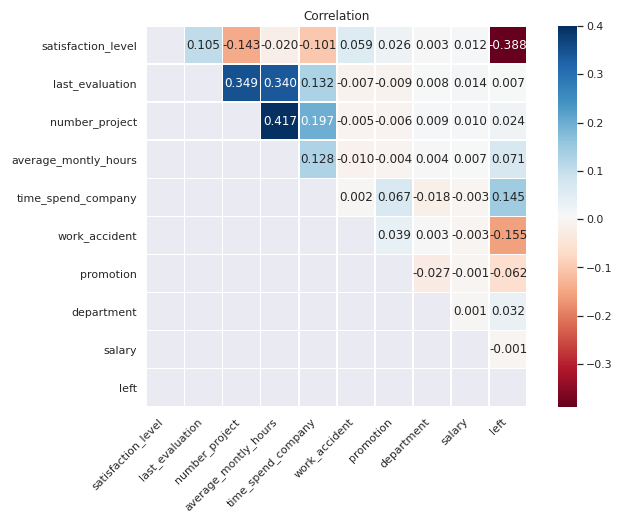
2.2. 相关性分析
根据热力图显示,可以发现:
满意度(satisfaction_level)- 员工满意度(satisfaction_level)离职(left)呈较大负相关(-)关系,与完成项目数(number_project)、在公司的年份(time_spend_company)也有一定的负相关性。
绩效评估(last_evaluation)- 上一次的绩效评估(last_evaluation)与完成项目数(number_project)和平均每月工作时间(average_montly_hours)这两个特征呈较大的正相关(+)关系,也就是说,完成项目数越多,平均每月工作时长越长,员工能获得更高的评价。
- 但绩效评估与工资,晋升都没有什么相关性,所以员工得到了高绩效评价也不会升职或者涨工资。
离职(left)- 离职率与员工满意度(satisfaction_level)、过去5年是否有晋升(promotion_last_5years)、是否有工伤(work_accident)、工资薪酬(salary)呈负相关(-)关系。如果员工对公司不太满意,且个人价值实现不高,那么离职的可能性会很大。
- 离职率与员工的在公司的年份(time_spend_company)呈较大正相关(+)关系。与平均每月工作时间(average_montly_hours),所在部门(department)也呈些许正相关性。
corr = df.corr()                 # pearson相关系数
mask = np.zeros_like(corr)
mask[np.tril_indices_from(mask)]=True
with sns.axes_style("white"):
    sns.set(rc={'figure.figsize':(11,7)})
    ax = sns.heatmap(corr,
                xticklabels=True, yticklabels=True,
                cmap='RdBu', # cmap='YlGnBu',  # 颜色
                mask=mask,   # 使用掩码只绘制矩阵的一部分
                fmt='.3f',     # 格式设置
                annot=True,    # 方格内写入数据
                linewidths=.5, # 热力图矩阵之间的间隔大小
                vmax=.4,       # 图例中最大值
                square = True
                # center = 0
                )

plt.title("Correlation")
label_x = ax.get_xticklabels()
plt.setp(label_x,rotation=45, horizontalalignment='right')
plt.show()
2.3.变量分析
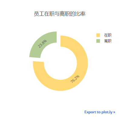
2.3.1. 公司当前员工离职与在职的比率
left_count = df['left'].value_counts().reset_index(name = "left_count")
trace = Pie(labels = ['在职','离职'], values = left_count.left_count,
            hoverinfo = "labels + percent + name",
            marker = dict(colors = colors[3:]), hole = .6, pull = .1)
layout = Layout(title = "员工在职与离职的比率", width = 380, height = 380)
iplot(Figure(data = [trace], layout = layout))
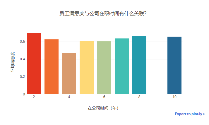
2.3.2. 公司员工的满意度与入职年份的关系
time_mean_satifaction = df.groupby(by = ['time_spend_company'])['satisfaction_level'].mean().reset_index(name = "average_satisfaction") # 取满意度的均值的
trace = Bar(x=time_mean_satifaction.time_spend_company, y=time_mean_satifaction.average_satisfaction, marker=dict(color = colors),)
layout = Layout(title= "员工满意度与公司在职时间有什么关联?",
                width = 700, height = 400,
                xaxis = dict(title="在公司时间(年)"),
                yaxis = dict(title = "平均满意度"),
                )
iplot(Figure(data=[trace],layout= layout))
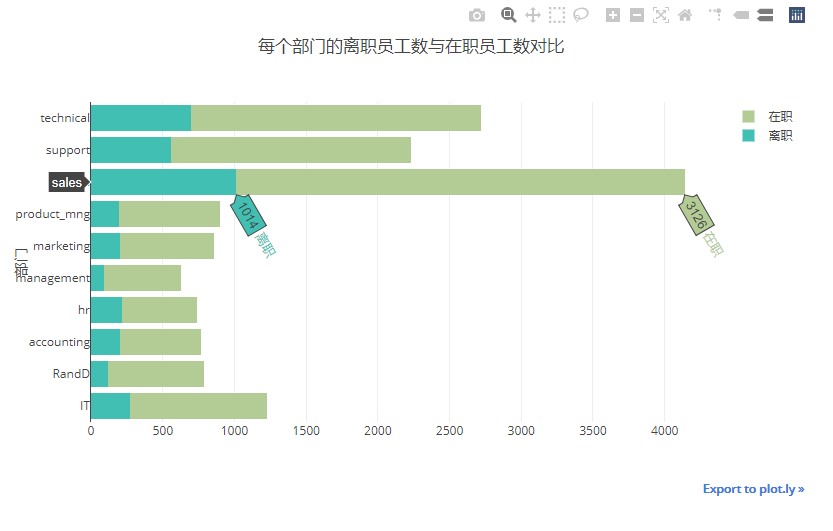
2.3.3. 公司各部门的员工离职与在职情况对比
可以看出,sales部门的离职人数最多,有1014人,其次是technical技术部门离职697人。
depart_left_table = pd.crosstab(index=df['department'],columns=df['left'])
data = []
left_eles = df.left.unique()
for l in left_eles:
    trace = Bar(x = depart_left_table[l], y = depart_left_table.index, name=('离职' if l == 1 else '在职'),orientation='h',marker=dict(color=colors[l+4]))
    data.append(trace)
layout = Layout(title="每个部门的离职员工数与在职员工数对比", barmode="stack",width=800,height=500,yaxis=dict(title="部门",tickmode="array",tickvals=list(department_dict.keys()),ticktext=list(department_dict.values())))
iplot(Figure(data= data, layout=layout))
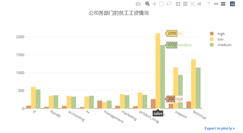
2.3.4. 公司各部门的员工的工资水平
销售部门(sales)低工资水平(low salary)的最多,有2099人,其次是技术部门(technical)与后勤部门(support),分别为1372人与1146人。
depart_salary_table = pd.crosstab(index=df['department'], columns=df['salary'])
# depart_salary_table
data = []
for i in range(3):
    trace = Bar(x=depart_salary_table.index, y=depart_salary_table[i],name=salary_dict[i],marker=dict(color=colors[i+2]))
    data.append(trace)
layout = Layout(title="公司各部门的员工工资情况",width=800,height=450,xaxis = dict(tickmode="array",tickvals=list(department_dict.keys()),ticktext=list(department_dict.values())))
iplot(Figure(data = data,layout = layout))
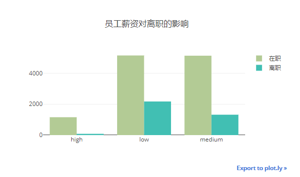
2.3.5 员工薪资与离职率
低薪与中等薪资的员工离职率偏高分别是42%,26%,高薪员工只用7%的离职率。
salary_left_table=pd.crosstab(index=df['salary'],columns=df['left'])
data = []
for i in range(2):
    trace = Bar(x=salary_left_table.index, y=salary_left_table[i],name=("在职" if i ==0 else "离职"),marker=dict(color=colors[i+4]))
    data.append(trace)
layout = Layout(title="员工薪资对离职的影响",width=580,height=350,xaxis = dict(tickmode="array",tickvals=list(salary_dict.keys()),ticktext=list(salary_dict.values())))
iplot(Figure(data = data,layout = layout))
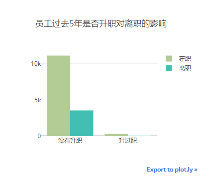
2.3.6. 员工过去5年的升职情况与离职对比
过去5年都没有升过职的员工离职率相比升过职的要高出很多。升过职的员工94%都在职。
promotion_left_table=pd.crosstab(index=df['promotion'],columns=df['left'])
promotion_dict = {0:"没有升职",1:"升过职"}
data = []
for i in range(2):
    trace = Bar(x=promotion_left_table.index, y=promotion_left_table[i],name=("在职" if i ==0 else "离职"),marker=dict(color=colors[i+4]))
    data.append(trace)
layout = Layout(title="员工过去5年是否升职对离职的影响",width=400,height=350,xaxis = dict(tickmode="array",tickvals=list(promotion_dict.keys()),ticktext=list(promotion_dict.values())))
iplot(Figure(data = data,layout = layout))
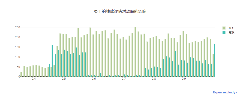
2.3.7. 员工绩效与离职的对比
离职员工不乏很多获得高度评价的
eva_left_table = pd.crosstab(index=df['last_evaluation'], columns=df['left'])
data = []
for i in range(2):
    trace = Bar(x=eva_left_table.index, y=eva_left_table[i],name=("在职" if i ==0 else "离职"),marker=dict(color=colors[i+4]))
    data.append(trace)
layout = Layout(title="员工的绩效评估对离职的影响",width=1000,height=400,)#xaxis = dict(tickmode="array",tickvals=list(promotion_dict.keys()),ticktext=list(promotion_dict.values())))
iplot(Figure(data = data,layout = layout))
3.总结
3.1. 离职原因分析
根据上面的👆分析,总的来看,离职员工的特征有以下几点:
- 对公司满意度低;
- 平均每天工作时长为10.4个小时(按一个月每周工作5天来计算),工作劳累;
- 薪资大多为中低水平;
- 过去5年基本没有升过职;
- 离职员工大部分来自销售、技术与后勤部门,销售部门占主要;
- 员工离职并不是单纯的因为绩效不好,相反,有一大半的离职员工的绩效评价都很高,在0.8-1之间都存在。结合之前相关性分析的发现,高绩效并不会带来升职和加薪,这也从侧面说明了为什么许多获得高评价的员工也会离职的原因。
所以,公司里大部分员工离职是因为满意度低、工资低、个人价值实现得不到满足。
3.2. 公司需要思考🤔的问题
- 为什么获得高绩效评价的员工离职率也很高?甚至评价最高的离职员工数有170多人?为什么这部分员工等不到升职与加薪?
- 为什么销售部门的离职员工最多?
- 为什么员工对公司的满意度低?
公司应该为员工创造一个良好的工作氛围,待遇与职业发展,更大限度的让员工实现自身的价值,从而更好的留住员工。
参考
[1]https://www.kaggle.com/mizanhadi/hr-employee-data-visualisation

魔乐社区(Modelers.cn) 是一个中立、公益的人工智能社区,提供人工智能工具、模型、数据的托管、展示与应用协同服务,为人工智能开发及爱好者搭建开放的学习交流平台。社区通过理事会方式运作,由全产业链共同建设、共同运营、共同享有,推动国产AI生态繁荣发展。
更多推荐


 6
6 0
0- 0


 已为社区贡献1条内容

所有评论(0)