LeNet实现

import torch
from torch import nn
from d2l import torch as d2l

class Reshape(torch.nn.Module):
    def forward(self,x):
        # view用来reshape，-1这一维由计算得出，1单通道
        return x.view(-1,1,28,28)
    
net=nn.Sequential(
    # reshape层。原来的图片是32*32的已经padding好了，现在28*28把padding删除了
    Reshape(),
    # 2维卷积，1输入通道数，6输出通道数，5x5,(28+2+2-5+1)/1=28
    # 常用卷积核大小2x2,5x5,7x7,11x11；padding=核大小/2,为了降低输出的shape
    nn.Conv2d(1,6,kernel_size=5,padding=2),
    # 激活函数，非线性单元，可以由简单函数模拟复杂函数的关键
    nn.Sigmoid(),
    # 作用，降低卷积对位置的敏感度，一般放到卷积层之后
    # 池化层对每个通道单独做池化，不改变通道数量
    # (28+0+0-2+2)/2=16，通过stride减半输出shape
    nn.AvgPool2d(kernel_size=2,stride=2),
    # 6输入通道数，16输出通道数，通过增加输出通道保留信息
    # (16+0+0-5+1)/1=10,stride默认就是1
    nn.Conv2d(6,16,kernel_size=5),
    nn.Sigmoid(),
    # (10+0+0-2+2)/2=5
    nn.AvgPool2d(kernel_size=2,stride=2),
    # 展平层，展平之后才能进行全连接
    nn.Flatten(),
    # 通道数16*5*5，(输入单元数量，输出单元数量)
    nn.Linear(16*5*5,120),
    nn.Sigmoid(),
    nn.Linear(120,84),
    nn.Sigmoid(),
    nn.Linear(84,10)
)

# 检查模型
# ！1个输入,1个通道，28*28的图片
# ！4个括号4个维度，shape看括号里面的元素数量
X=torch.rand(size=(1,1,28,28),dtype=torch.float32)
for layer in net:
    X=layer(X)
    print(layer.__class__.__name__,'output shape:\t',X.shape)

Reshape output shape:	 torch.Size([1, 1, 28, 28])
Conv2d output shape:	 torch.Size([1, 6, 28, 28])
Sigmoid output shape:	 torch.Size([1, 6, 28, 28])
AvgPool2d output shape:	 torch.Size([1, 6, 14, 14])
Conv2d output shape:	 torch.Size([1, 16, 10, 10])
Sigmoid output shape:	 torch.Size([1, 16, 10, 10])
AvgPool2d output shape:	 torch.Size([1, 16, 5, 5])
Flatten output shape:	 torch.Size([1, 400])
Linear output shape:	 torch.Size([1, 120])
Sigmoid output shape:	 torch.Size([1, 120])
Linear output shape:	 torch.Size([1, 84])
Sigmoid output shape:	 torch.Size([1, 84])
Linear output shape:	 torch.Size([1, 10])

# ！4个括号4个维度，shape看括号里面的元素数量
# 第1个括号里面1个元素，第2个括号里面2个元素，第3个括号里面2个元素，第3个括号里面2个元素
torch.tensor([[
    [
        [1,2],
        [3,4]
    ],
    [
        [1,2],
        [3,4]
    ]
]]).shape

torch.Size([1, 2, 2, 2])

LeNet在Fashion-MNIST数据集上的表现

batch_size=256
train_iter,test_iter=d2l.load_data_fashion_mnist(batch_size=batch_size)

修改评估函数，在gpu上运行模型

def evaluate_accuracy_gpu(net,data_iter,device=None):
    '''
    评估精度，在gpu上运行模型
    :return 平均精度=总精度/输出元素数量
    '''
    if isinstance(net,nn.Module):
        # ！！模型评估
        net.eval()
        # 如果device=None，没有给定设备，看第1个参数在那个设备上
        if not device:
            # net.Parameters()是可迭代对象
            # next(iter(可迭代对象))获取可迭代对象的下1个值
            # 这里next只调用了1次，就获取了第1个参数
            # 迭代所有的参数获取每个参数的设备
            device=next(iter(net.parameters())).device
    # 创建2个维度的累加器
    metric=d2l.Accumulator(2)
    # 评估模型时不需要计算梯度
    # 上下文管理器
    # 进入with语句时自动调用__enter__()魔术方法
    # 退出with语句时自动调用__exit__()魔术方法
    with torch.no_grad():
        for X,y in data_iter:
            # 如果X是list类型
            if isinstance(X,list):
                # 以这种方式放入device
                X=[x.to(device) for x in X]
            else:
                # 否则以这种方式放入device
                X=X.to(device)
            y=y.to(device)
            # numel() 元素数量
            metric.add(d2l.accuracy(net(X),y),y.numel())
    # 平均精度=总精度/输出元素数量
    return metric[0]/metric[1]

修改训练函数，在gpu上训练模型

def train_ch6(net,train_iter,test_iter,num_epochs,lr,device):
    '''
    在gpu上训练模型(在第六章定义)
    '''
    def init_weights(m):
        if type(m)==nn.Linear or type(m)==nn.Conv2d:
            # 数值稳定性，防止梯度爆炸和梯度消失
            # 数值稳定性，前向每一层输出的方差应该尽量相等，后向梯度的方差应该尽量相等
            # 数值稳定性，稳定输入输出，让每层的输出的方差差不多，防止开始训练时模型就梯度爆炸或消失
            # 数值稳定性
            # - 正向每层输出期望=0，方差为常数
            # - 反向每层梯度期望=0，方差为常数
            # xavier参数初始化，提高数值稳定性，防止梯度爆炸或消失
            # - 数值稳定性，每一层输出的方差应该尽量相等，为此，每层的权重应该满足哪些条件
            # - xavier参数初始化，防止梯度爆炸或消失
            # - 限制参数的选择范围，使得最终的函数曲线更平滑，泛化能力更强
            # - 它表示权重和梯度期望=0，权重和梯度的方差由第t层输入和输出的神经元数量决定
            nn.init.xavier_uniform_(m.weight)
    net.apply(init_weights)
    print('training on', device)
    # 将模型放到GPU上
    net.to(device)
    # 优化函数
    optimizer = torch.optim.SGD(net.parameters(), lr=lr)
    # 损失函数，交叉熵
    loss = nn.CrossEntropyLoss()
    # 动画展示损失函数
    animator = d2l.Animator(xlabel='epoch', 
                xlim=[1, num_epochs],
                legend=['train loss', 'train acc', 'test acc'])
    # num_batches总批量数
    timer, num_batches = d2l.Timer(), len(train_iter)
    for epoch in range(num_epochs):
        metric = d2l.Accumulator(3)
        # ！！训练
        net.train()
        # 获取索引i而使用枚举enumerate
        for i, (X, y) in enumerate(train_iter):
            timer.start()
            # ！清空梯度，默认会梯度累积
            optimizer.zero_grad()
            # ！数据放到gpu上
            # 在计算之前放到gpu上
            X, y = X.to(device), y.to(device)
            # ！前向传播，魔法函数自动调用forward()
            y_hat = net(X)
            # ！计算损失
            l = loss(y_hat, y)
            # ！后向传播
            l.backward()
            # ！优化1步
            optimizer.step()
            # 记录训练过程不需要计算梯度
            # 什么时候不能计算梯度，需要梯度的变量在非训练步骤中不能计算梯度
            with torch.no_grad():
                metric.add(l * X.shape[0], d2l.accuracy(y_hat, y), X.shape[0])
            timer.stop()
            # l=loss，训练损失*样本数量/样本数量=训练损失
            train_l = metric[0] / metric[2]
            # 匹配label数量/样本数量=训练精度
            train_acc = metric[1] / metric[2]
            # //下取整，训练5个批量或到最后1个批量时输出1次
            if (i + 1) % (num_batches // 5) == 0 or i == num_batches - 1:
                animator.add(epoch + (i + 1) / num_batches,
                             (train_l, train_acc, None))
        # 1epoch，验证1次平均精度
        test_acc = evaluate_accuracy_gpu(net, test_iter) 
        # 绘图
        animator.add(epoch + 1, (None, None, test_acc))
    # l=loss
    print(f'loss {train_l:.3f}, train acc {train_acc:.3f}, '
          f'test acc {test_acc:.3f}')
    # 耗时 样本总数量/耗时，1s中训练多少个样本
    print(f'{metric[2] * num_epochs / timer.sum():.1f} examples/sec '
          f'on {str(device)}')

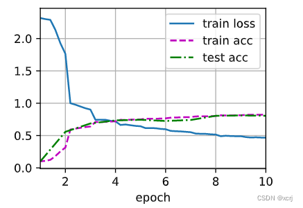
开始训练

# 没有overfitting可能就是underfitting
lr, num_epochs = 0.9, 10
train_ch6(net, train_iter, test_iter, num_epochs, lr, d2l.try_gpu())

loss 0.467, train acc 0.824, test acc 0.807
48045.4 examples/sec on cuda:0

总结
涉及

• 数据（训练集 验证集合，测试集合）
• 模型
• 超参数
• 损失函数
• 优化函数 优化损失函数，获取模型参数
• 训练
• 评估

过程

• num_epochs
• 获取batch_size数据
• 数据放到设备上
• 前向传播
• 计算损失函数值
• 后向传播
• 优化函数优化1步

模型超参数

• 卷积层：kernel_size，padding，stride，channel
• 池化层：kernel_size，padding，stride

超参数

• num_epochs
• batch_size
• lr

正则化超参数

• weight_decay
• p 丢弃概率

没有overfitting可能就是underfitting

• overfitting后可以通过某些方式调整

query

卷积层的输出将输入宽高减半，通道数增加1倍

• 答：将抽象后的信息保存到了通道中。同样的1个像素保存了更多信息，更多的通道作用到了这1个像素中

view和reshape的区别

• 答：reshape的功能比view更强大。view视图是原有tensor的视图，不开辟新的存储空间，返回原有存储空间的引用。view只适用于连续性的tensor

6通道到16通道

• 答：16x6x二维卷积核

poloclub.github.io/cnn-explainer/

• 答：可视化cnn学到的东西