计算机视觉目标检测——DETR代码解读
本周主要对DETR(End-to-End Object Detection with Transformers)的代码实现进行了详细解读和学习。DETR是首个将目标检测任务转化为集合预测问题的端到端框架,通过Transformer的全局建模能力,显著简化了检测器的设计。在代码解读中,重点分析了DETR的整体架构,包括CNN特征提取、正余弦位置编码、Transformer的Encoder-Decod
计算机视觉目标检测——DETR代码解读
文章目录
摘要
本周主要对DETR(End-to-End Object Detection with Transformers)的代码实现进行了详细解读和学习。DETR是首个将目标检测任务转化为集合预测问题的端到端框架,通过Transformer的全局建模能力,显著简化了检测器的设计。在代码解读中,重点分析了DETR的整体架构,包括CNN特征提取、正余弦位置编码、Transformer的Encoder-Decoder结构和基于集合预测的损失函数。Transformer模块通过多头注意力机制构建全局上下文关系,而损失函数利用匈牙利算法实现预测框与真实框的一对一匹配,避免了传统方法中的NMS后处理。代码展示了DETR在架构上的高效性与简洁性。
Abstract
This week’s work focused on a comprehensive analysis of the code implementation for DETR (End-to-End Object Detection with Transformers). DETR represents a pioneering framework that reformulates object detection as a set prediction task, eliminating the need for post-processing steps like NMS. The study explored the overall architecture of DETR, including CNN-based feature extraction, sine positional encoding, the Transformer-based encoder-decoder structure, and the set prediction loss function. The Transformer module leverages multi-head attention mechanisms to establish global contextual relationships, while the loss function employs the Hungarian algorithm to achieve one-to-one matching between predicted and ground-truth boxes. The code demonstrates the efficiency and simplicity of DETR’s design.
一、DETR代码解读
1. 整体代码
1.1 整体架构
先回顾一下DETR的整体框架:
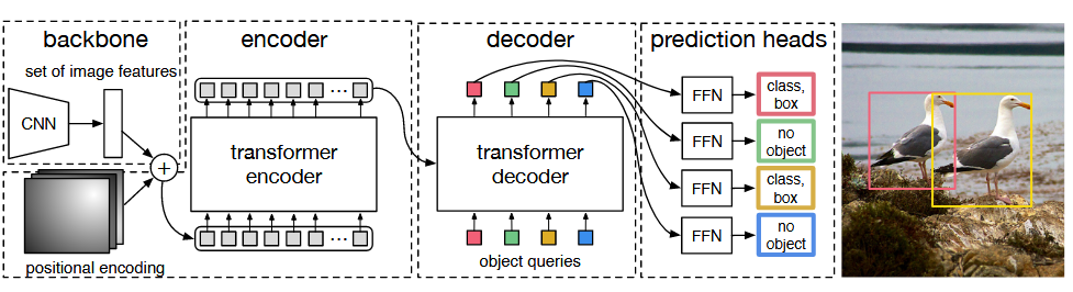
DETR的网络结构主要由三部分组成:CNN骨干网、Transformer编码器和解码器,以及输出层。
- CNN骨干网:负责从输入图像中提取特征图。DETR通常使用ResNet等深度卷积神经网络作为骨干网,通过一系列的卷积和池化操作,将输入图像转换为高维特征图。
- Transformer编码器:用于对CNN骨干网提取的特征图进行编码。编码器由多个Transformer block组成,每个block包含自注意力层和前馈神经网络层。通过多层自注意力机制,编码器能够捕获特征图中不同位置之间的全局上下文关系,生成一组特征向量。
- Transformer解码器:解码器是DETR实现集合预测的关键部分。它接受编码器的输出和一组可学习的目标查询(object queries),通过自注意力机制和编码器-解码器注意力机制,将目标查询解码为一系列目标的边界框坐标和类别标签。
- 预测头:两个简单的前馈网络( feed forward network,FFN )来进行最终的检测预测。分别用于预测边界框的标准化中心坐标、高度和宽度,以及类别标签。
1.2 基于集合预测的损失函数
DETR在单次通过解码器时推断一个固定大小的有 N 个预测的集合,其中 N 被设置为显著大于图像中典型的物体数量,文中N为100。训练的主要困难之一是在 ground truth 方面对预测对象(类别、位置、大小)进行打分。我们的损失在预测对象和真实对象之间产生一个最佳的二分匹配,然后优化 object-specific ( bounding box ) 的损失。
用 y y y表示对象的ground truth集合, y ^ = { y ^ i } i = 1 N \hat y = \{ {\hat y_i}\} _{i = 1}^N y^={y^i}i=1N表示有 N N N个预测的集合。假设N远大于图像中物体的个数,我们考虑y也是一个大小为N的被 ( no object ) 填充的集合。为了在这两个集合之间找到一个二分匹配,我们用最低的代价搜索N个元素 σ ∈ ℘ N \sigma \in {\wp _N} σ∈℘N的一个置换:
σ ^ = arg min σ ∈ ℘ N ∑ i N L m a t c h ( y i , y ^ σ ( i ) ) \hat \sigma = \mathop {\arg \min }\limits_{\sigma \in {\wp _N}} \sum\limits_i^N {{L_{match}}({y_i},{{\hat y}_{\sigma (i)}})} σ^=σ∈℘Nargmini∑NLmatch(yi,y^σ(i))
-
L m a t c h ( y i , y ^ σ ( i ) ) {{L_{match}}({y_i},{{\hat y}_{\sigma (i)}})} Lmatch(yi,y^σ(i))是真值 y i {{y_i}} yi和具有索引 σ i {\sigma _i} σi的一个预测之间的一个成对匹配代价(a pair-wise matching cost)。这个最优分配是通过匈牙利算法计算的。匹配代价同时考虑了类预测以及预测框和真实框之间的相似性。
-
真实集合的每个元素 i i i都可以看成一个 y i = ( c i , b i ) {y_i} = ({c_i},{b_i}) yi=(ci,bi),其中 c i {c_i} ci是目标类标签(目标类标签特可能是 ϕ \phi ϕ)。 b i ∈ [ 0 , 1 ] 4 {b_i} \in {\left[ {0,1} \right]^4} bi∈[0,1]4是一个向量,它定义了真实框的中心坐标及其相对于图像的高度和宽度。
-
对于索引 σ i {\sigma _i} σi的预测,我们定义类 c i {c _i} ci的概率为 p ^ σ ( i ) ( c i ) {{\hat p}_{\sigma (i)}}({c_i}) p^σ(i)(ci),预测框为 b ^ σ ( i ) {{\hat b}_{\sigma (i)}} b^σ(i)。
利用上述的符号,可以将 L m a t c h ( y i , y ^ σ ( i ) ) {{L_{match}}({y_i},{{\hat y}_{\sigma (i)}})} Lmatch(yi,y^σ(i))定义为:
− 1 { c i ≠ ϕ } p ^ σ ( i ) ( c i ) + 1 { c i ≠ ϕ } L b o x ( b i , b ^ σ ( i ) ) - {1_{\{ {c_i} \ne \phi \} }}{{\hat p}_{\sigma (i)}}({c_i}) + {1_{\{ {c_i} \ne \phi \} }}{L_{box}}({b_i},{{\hat b}_{\sigma (i)}}) −1{ci=ϕ}p^σ(i)(ci)+1{ci=ϕ}Lbox(bi,b^σ(i))
其损失函数是计算上一步中匹配的所有配对的匈牙利损失。我们定义的损失类似于常见目标检测器的损失,即类别预测的负对数和box 损失的线性组合:
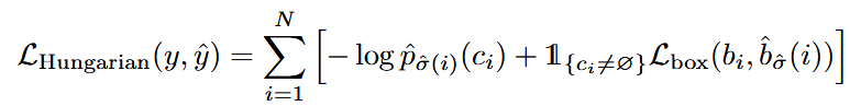
其中的 σ ^ {\hat \sigma } σ^是第一步中计算的最优分配。
1.3 论文中的示例代码
import torch
from torch import nn
from torchvision.models import resnet50

class DETR(nn.Module):
    def __init__(self, num_classes, hidden_dim, nheads, num_encoder_layers, num_decoder_layers):
        super().__init__()
        # backbone = resnet50 除掉average pool和fc层  只保留conv1 - conv5_x
        self.backbone = nn.Sequential(*list(resnet50(pretrained=True).children())[:-2])
        # 1x1卷积降维 2048->256
        self.conv = nn.Conv2d(2048, hidden_dim, 1)
        # 6层encoder + 6层decoder    hidden_dim=256  nheads多头注意力机制 8头   num_encoder_layers=num_decoder_layers=6
        self.transformer = nn.Transformer(hidden_dim, nheads, num_encoder_layers, num_decoder_layers)
        # 分类头
        self.linear_class = nn.Linear(hidden_dim, num_classes + 1)
        # 回归头
        self.linear_bbox = nn.Linear(hidden_dim, 4)
        # 位置编码  encoder输入
        self.row_embed = nn.Parameter(torch.rand(50, hidden_dim // 2))
        self.col_embed = nn.Parameter(torch.rand(50, hidden_dim // 2))
        # query pos编码  decoder输入
        self.query_pos = nn.Parameter(torch.rand(100, hidden_dim))


    def forward(self, inputs):
        x = self.backbone(inputs)    # [1,3,800,1066] -> [1,2048,25,34]
        h = self.conv(x)             # [1,2048,25,34] -> [1,256,25,34]
        H, W = h.shape[-2:]          # H=25  W=34
        # pos = [850,1,256]  self.col_embed = [50,128]  self.row_embed[:H]=[50,128]
        pos = torch.cat([self.col_embed[:W].unsqueeze(0).repeat(H, 1, 1),
                        self.row_embed[:H].unsqueeze(1).repeat(1, W, 1),
                        ], dim=-1).flatten(0, 1).unsqueeze(1)
        # encoder输入  decoder输入
        h = self.transformer(pos + h.flatten(2).permute(2, 0, 1), self.query_pos.unsqueeze(1))
        return self.linear_class(h), self.linear_bbox(h).sigmoid()


detr = DETR(num_classes=91, hidden_dim=256, nheads=8, num_encoder_layers=6, num_decoder_layers=6)
detr.eval()
inputs = torch.randn(1, 3, 800, 1066)
logits, bboxes = detr(inputs)
print(logits.shape)   # torch.Size([100, 1, 92])
print(bboxes.shape)   # torch.Size([100, 1, 4])
论文原文给出的代码,mAP只有40,虽然比真实的源码低了2个点,但是代码很简单,只有40多行,方便我们了解整个DETR的网络结构,可以与上述的DETR框架一一对应起来。
2. Backbone代码
整个Backbone主要包括CNN特征提取和位置编码两个部分。
首先是调用models/Backbone.py中的build_backbone函数创建Backbone:
def build_backbone(args):
    # 搭建backbone
    # 位置编码  PositionEmbeddingSine()
    position_embedding = build_position_encoding(args)
    train_backbone = args.lr_backbone > 0   # 是否需要训练backbone  True
    return_interm_layers = args.masks       # 是否需要返回中间层结果 目标检测False  分割True
    # 生成backbone  resnet50
    backbone = Backbone(args.backbone, train_backbone, return_interm_layers, args.dilation)
    # 将backbone输出与位置编码相加   0: backbone   1: PositionEmbeddingSine()
    model = Joiner(backbone, position_embedding)
    model.num_channels = backbone.num_channels   # 512
    return model
这里首先调用build_position_encoding函数生成正余弦位置编码position_embedding:[bs,256,H/32, W/32],其中256前128是y方向位置编码,后128是x方向位置编码;再调用Backbone类生成ResNet50对输入数据进行特征提取得到特征图[bs,2048,H/32, W/32]。最后Joiner将两者合并存储起来,方便后续使用。
2.1 CNN特征提取部分代码
创建ResNet50,先调用Backbone类:
class Backbone(BackboneBase):
    """ResNet backbone with frozen BatchNorm."""
    def __init__(self, name: str,
                 train_backbone: bool,
                 return_interm_layers: bool,
                 dilation: bool):
        # 直接调包 调用torchvision.models中的backbone
        backbone = getattr(torchvision.models, name)(
            replace_stride_with_dilation=[False, False, dilation],
            pretrained=is_main_process(), norm_layer=FrozenBatchNorm2d)
        # resnet50  2048
        num_channels = 512 if name in ('resnet18', 'resnet34') else 2048
        super().__init__(backbone, train_backbone, num_channels, return_interm_layers)
这个类是继承自BackboneBase类的,而且CNN直接调用的就是torchvision.models中的模型,所以直接看BackboneBase类:
class BackboneBase(nn.Module):

    def __init__(self, backbone: nn.Module, train_backbone: bool, num_channels: int, return_interm_layers: bool):
        super().__init__()
        for name, parameter in backbone.named_parameters():
            # layer0 layer1不需要训练 因为前面层提取的信息其实很有限 都是差不多的 不需要训练
            if not train_backbone or 'layer2' not in name and 'layer3' not in name and 'layer4' not in name:
                parameter.requires_grad_(False)
        # False 检测任务不需要返回中间层
        if return_interm_layers:
            return_layers = {"layer1": "0", "layer2": "1", "layer3": "2", "layer4": "3"}
        else:
            return_layers = {'layer4': "0"}
        # 检测任务直接返回layer4即可  执行torchvision.models._utils.IntermediateLayerGetter这个函数可以直接返回对应层的输出结果
        self.body = IntermediateLayerGetter(backbone, return_layers=return_layers)
        self.num_channels = num_channels

    def forward(self, tensor_list: NestedTensor):
        """
        tensor_list: pad预处理之后的图像信息
        tensor_list.tensors: [bs, 3, 608, 810]预处理后的图片数据 对于小图片而言多余部分用0填充
        tensor_list.mask: [bs, 608, 810] 用于记录矩阵中哪些地方是填充的(原图部分值为False,填充部分值为True)
        """
        # 取出预处理后的图片数据 [bs, 3, 608, 810] 输入模型中  输出layer4的输出结果 dict '0'=[bs, 2048, 19, 26]
        xs = self.body(tensor_list.tensors)
        # 保存输出数据
        out: Dict[str, NestedTensor] = {}
        for name, x in xs.items():
            m = tensor_list.mask  # 取出图片的mask [bs, 608, 810] 知道图片哪些区域是有效的 哪些位置是pad之后的无效的
            assert m is not None
            # 通过插值函数知道卷积后的特征的mask  知道卷积后的特征哪些是有效的  哪些是无效的
            # 因为之前图片输入网络是整个图片都卷积计算的 生成的新特征其中有很多区域都是无效的
            mask = F.interpolate(m[None].float(), size=x.shape[-2:]).to(torch.bool)[0]
            # out['0'] = NestedTensor: tensors[bs, 2048, 19, 26] + mask[bs, 19, 26]
            out[name] = NestedTensor(x, mask)
        # out['0'] = NestedTensor: tensors[bs, 2048, 19, 26] + mask[bs, 19, 26]
        return out
这个类还是在调用torchvision.models中的模型,然后再把预处理后的图片数据[bs, 3, 608, 810]和mask数据[bs, 608, 810]输入到模型中(这个图片数据是经过pad填充的数据,而mask数据就是记录这些图片哪些像素位置是pad的,为True,没用pad的真实有效数据就为False)。经过前向传播,再调用IntermediateLayerGetter函数把对应层特征图提取出来,得到原图32倍下采样的特征图[bs, 2048, 19, 26],以及这张特征图对应的mask[bs, 19, 26]。
2.2 位置编码部分代码
这里主要是调用models/position_encoding.py中的build_position_encoding函数创建位置编码:
def build_position_encoding(args):
    """
    创建位置编码
    args: 一系列参数  args.hidden_dim: transformer中隐藏层的维度   args.position_embedding: 位置编码类型 正余弦sine or 可学习learned
    """
    # N_steps = 128 = 256 // 2  backbone输出[bs,256,25,34]  256维度的特征
    # 而传统的位置编码应该也是256维度的, 但是detr用的是一个x方向和y方向的位置编码concat的位置编码方式  这里和ViT有所不同
    # 二维位置编码   前128维代表x方向位置编码  后128维代表y方向位置编码
    N_steps = args.hidden_dim // 2
    if args.position_embedding in ('v2', 'sine'):
        # TODO find a better way of exposing other arguments
        # [bs,256,19,26]  dim=1时  前128个是y方向位置编码  后128个是x方向位置编码
        position_embedding = PositionEmbeddingSine(N_steps, normalize=True)
    elif args.position_embedding in ('v3', 'learned'):
        position_embedding = PositionEmbeddingLearned(N_steps)
    else:
        raise ValueError(f"not supported {args.position_embedding}")

    return position_embedding
可以看到,源码是实现了两种位置编码,一种是正余弦绝对位置编码,不需要额外的参数学习,另一种是可学习绝对位置编码。原论文用的是正余弦绝对位置编码,而且代码也是默认使用这个的,所以这里主要介绍PositionEmbeddingSine类:
class PositionEmbeddingSine(nn.Module):
    """
    Absolute pos embedding, Sine.  没用可学习参数  不可学习  定义好了就固定了
    This is a more standard version of the position embedding, very similar to the one
    used by the Attention is all you need paper, generalized to work on images.
    """
    def __init__(self, num_pos_feats=64, temperature=10000, normalize=False, scale=None):
        super().__init__()
        self.num_pos_feats = num_pos_feats    # 128维度  x/y  = d_model/2
        self.temperature = temperature        # 常数 正余弦位置编码公式里面的10000
        self.normalize = normalize            # 是否对向量进行max规范化   True
        if scale is not None and normalize is False:
            raise ValueError("normalize should be True if scale is passed")
        if scale is None:
            # 这里之所以规范化到2*pi  因为位置编码函数的周期是[2pi, 20000pi]
            scale = 2 * math.pi  # 规范化参数 2*pi
        self.scale = scale

    def forward(self, tensor_list: NestedTensor):
        x = tensor_list.tensors   # [bs, 2048, 19, 26]  预处理后的 经过backbone 32倍下采样之后的数据  对于小图片而言多余部分用0填充
        mask = tensor_list.mask   # [bs, 19, 26]  用于记录矩阵中哪些地方是填充的(原图部分值为False,填充部分值为True)
        assert mask is not None
        not_mask = ~mask   # True的位置才是真实有效的位置

        # 考虑到图像本身是2维的 所以这里使用的是2维的正余弦位置编码
        # 这样各行/列都映射到不同的值 当然有效位置是正常值 无效位置会有重复值 但是后续计算注意力权重会忽略这部分的
        # 而且最后一个数字就是有效位置的总和,方便max规范化
        # 计算此时y方向上的坐标  [bs, 19, 26]
        y_embed = not_mask.cumsum(1, dtype=torch.float32)
        # 计算此时x方向的坐标    [bs, 19, 26]
        x_embed = not_mask.cumsum(2, dtype=torch.float32)

        # 最大值规范化 除以最大值 再乘以2*pi 最终把坐标规范化到0-2pi之间
        if self.normalize:
            eps = 1e-6
            y_embed = y_embed / (y_embed[:, -1:, :] + eps) * self.scale
            x_embed = x_embed / (x_embed[:, :, -1:] + eps) * self.scale

        dim_t = torch.arange(self.num_pos_feats, dtype=torch.float32, device=x.device)   # 0 1 2 .. 127
        # 2i/2i+1: 2 * (dim_t // 2)  self.temperature=10000   self.num_pos_feats = d/2
        dim_t = self.temperature ** (2 * (dim_t // 2) / self.num_pos_feats)   # 分母

        pos_x = x_embed[:, :, :, None] / dim_t   # 正余弦括号里面的公式
        pos_y = y_embed[:, :, :, None] / dim_t   # 正余弦括号里面的公式
        # x方向位置编码: [bs,19,26,64][bs,19,26,64] -> [bs,19,26,64,2] -> [bs,19,26,128]
        pos_x = torch.stack((pos_x[:, :, :, 0::2].sin(), pos_x[:, :, :, 1::2].cos()), dim=4).flatten(3)
        # y方向位置编码: [bs,19,26,64][bs,19,26,64] -> [bs,19,26,64,2] -> [bs,19,26,128]
        pos_y = torch.stack((pos_y[:, :, :, 0::2].sin(), pos_y[:, :, :, 1::2].cos()), dim=4).flatten(3)
        # concat: [bs,19,26,128][bs,19,26,128] -> [bs,19,26,256] -> [bs,256,19,26]
        pos = torch.cat((pos_y, pos_x), dim=3).permute(0, 3, 1, 2)

        # [bs,256,19,26]  dim=1时  前128个是y方向位置编码  后128个是x方向位置编码
        return pos
可以对照公式:
P E ( p o s , 2 i ) = sin ( p o s / 1000 0 2 i / d m o d e l ) P{E_{(pos,2i)}} = \sin (pos/{10000^{2i/{d_{\bmod el}}}}) PE(pos,2i)=sin(pos/100002i/dmodel)
P E ( p o s , 2 i + 1 ) = cos ( p o s / 1000 0 2 i / d m o d e l ) P{E_{(pos,2i + 1)}} = \cos (pos/{10000^{2i/{d_{\bmod el}}}}) PE(pos,2i+1)=cos(pos/100002i/dmodel)
3. Transfomer代码
先看下调用接口:
def build_transformer(args):
    return Transformer(
        d_model=args.hidden_dim,
        dropout=args.dropout,
        nhead=args.nheads,
        dim_feedforward=args.dim_feedforward,
        num_encoder_layers=args.enc_layers,
        num_decoder_layers=args.dec_layers,
        normalize_before=args.pre_norm,
        return_intermediate_dec=True,
    )
直接调用Transformer类:
class Transformer(nn.Module):

    def __init__(self, d_model=512, nhead=8, num_encoder_layers=6,
                 num_decoder_layers=6, dim_feedforward=2048, dropout=0.1,
                 activation="relu", normalize_before=False,
                 return_intermediate_dec=False):
        super().__init__()
        """
        d_model: 编码器里面mlp(前馈神经网络  2个linear层)的hidden dim 512
        nhead: 多头注意力头数 8
        num_encoder_layers: encoder的层数 6
        num_decoder_layers: decoder的层数 6
        dim_feedforward: 前馈神经网络的维度 2048
        dropout: 0.1
        activation: 激活函数类型 relu
        normalize_before: 是否使用前置LN
        return_intermediate_dec: 是否返回decoder中间层结果  False
        """
        # 初始化一个小encoder
        encoder_layer = TransformerEncoderLayer(d_model, nhead, dim_feedforward,
                                                dropout, activation, normalize_before)
        encoder_norm = nn.LayerNorm(d_model) if normalize_before else None
        # 创建整个Encoder层  6个encoder层堆叠
        self.encoder = TransformerEncoder(encoder_layer, num_encoder_layers, encoder_norm)

        # 初始化一个小decoder
        decoder_layer = TransformerDecoderLayer(d_model, nhead, dim_feedforward,
                                                dropout, activation, normalize_before)
        decoder_norm = nn.LayerNorm(d_model)
        # 创建整个Decoder层  6个decoder层堆叠
        self.decoder = TransformerDecoder(decoder_layer, num_decoder_layers, decoder_norm,
                                          return_intermediate=return_intermediate_dec)

        # 参数初始化
        self._reset_parameters()

        self.d_model = d_model  # 编码器里面mlp的hidden dim 512
        self.nhead = nhead      # 多头注意力头数 8

    def _reset_parameters(self):
        for p in self.parameters():
            if p.dim() > 1:
                nn.init.xavier_uniform_(p)

    def forward(self, src, mask, query_embed, pos_embed):
        """
        src: [bs,256,19,26] 图片输入backbone+1x1conv之后的特征图
        mask: [bs, 19, 26]  用于记录特征图中哪些地方是填充的(原图部分值为False,填充部分值为True)
        query_embed: [100, 256]  类似于传统目标检测里面的anchor  这里设置了100个   需要预测的目标
        pos_embed: [bs, 256, 19, 26]  位置编码
        """
        # bs  c=256  h=19  w=26
        bs, c, h, w = src.shape
        # src: [bs,256,19,26]=[bs,C,H,W] -> [494,bs,256]=[HW,bs,C]
        src = src.flatten(2).permute(2, 0, 1)
        # pos_embed: [bs, 256, 19, 26]=[bs,C,H,W] -> [494,bs,256]=[HW,bs,C]
        pos_embed = pos_embed.flatten(2).permute(2, 0, 1)
        # query_embed: [100, 256]=[num,C] -> [100,bs,256]=[num,bs,256]
        query_embed = query_embed.unsqueeze(1).repeat(1, bs, 1)
        # mask: [bs, 19, 26]=[bs,H,W] -> [bs,494]=[bs,HW]
        mask = mask.flatten(1)

        # tgt: [100, bs, 256] 需要预测的目标query embedding 和 query_embed形状相同  且全设置为0
        #                     在每层decoder层中不断的被refine,相当于一次次的被coarse-to-fine的过程
        tgt = torch.zeros_like(query_embed)
        # memory: [494, bs, 256]=[HW, bs, 256]  Encoder输出  具有全局相关性(增强后)的特征表示
        memory = self.encoder(src, src_key_padding_mask=mask, pos=pos_embed)
        # [6, 100, bs, 256]
        # tgt:需要预测的目标 query embeding
        # memory: encoder的输出
        # pos: memory的位置编码
        # query_pos: tgt的位置编码
        hs = self.decoder(tgt, memory, memory_key_padding_mask=mask,
                          pos=pos_embed, query_pos=query_embed)
        # decoder输出 [6, 100, bs, 256] -> [6, bs, 100, 256]
        # encoder输出 [bs, 256, H, W]
        return hs.transpose(1, 2), memory.permute(1, 2, 0).view(bs, c, h, w)
仔细分析这个类会发现,我们虽然暂时不了解模型的细节部分,但是模型的主体框架已经定义出来了。整个Transformer其实就是输入经过Backbone输出的特征图src(降维到256)、src_key_padding_mask(记录特征图每个位置是否是被pad的,pad的就不需要计算注意力)和位置编码pos到TransformerEncoder中,而TransformerEncoder其实是由TransformerEncoderLayer组成的;然后再输入encoder的输出、mask、位置编码和query编码到TransformerEncoder中,而TransformerEncoder是由TransformerDecoderLayer组成的。
所以,下面分为TransformerEncoder和TransformerDecoder两个模块来了解Transformer具体细节组成。
3.1 TransformerEncoder代码
这个部分就是调用_get_clones函数,复制6份TransformerEncoderLayer类,然后前向传播依次输入这6个TransformerEncoderLayer类,不断的计算特征图的自注意力,并不断的增强特征图,最终得到最强的(信息最多的)特征图output:[h*w, bs, 256]。值得注意的是,整个TransformerEncoder过程特征图的shape是不变的。
class TransformerEncoder(nn.Module):

    def __init__(self, encoder_layer, num_layers, norm=None):
        super().__init__()
        # 复制num_layers=6份encoder_layer=TransformerEncoderLayer
        self.layers = _get_clones(encoder_layer, num_layers)
        # 6层TransformerEncoderLayer
        self.num_layers = num_layers
        self.norm = norm  # layer norm

    def forward(self, src,
                mask: Optional[Tensor] = None,
                src_key_padding_mask: Optional[Tensor] = None,
                pos: Optional[Tensor] = None):
        """
        src: [h*w, bs, 256]  经过Backbone输出的特征图(降维到256)
        mask: None
        src_key_padding_mask: [h*w, bs]  记录每个特征图的每个位置是否是被pad的(True无效   False有效)
        pos: [h*w, bs, 256] 每个特征图的位置编码
        """
        output = src

        # 遍历这6层TransformerEncoderLayer
        for layer in self.layers:
            output = layer(output, src_mask=mask,
                           src_key_padding_mask=src_key_padding_mask, pos=pos)

        if self.norm is not None:
            output = self.norm(output)

        # 得到最终ENCODER的输出 [h*w, bs, 256]
        return output

def _get_clones(module, N):
    return nn.ModuleList([copy.deepcopy(module) for i in range(N)])
我们来看一下TransformerEncoderLayer:
下图是TransformerEncoderLayer的结构:Encoder Layer = multi-head Attention + add&Norm + feed forward + add&Norm,重点在于multi-head Attention。

class TransformerEncoderLayer(nn.Module):

    def __init__(self, d_model, nhead, dim_feedforward=2048, dropout=0.1,
                 activation="relu", normalize_before=False):
        super().__init__()
        """
        小encoder层  结构:multi-head Attention + add&Norm + feed forward + add&Norm
        d_model: mlp 前馈神经网络的dim
        nhead: 8头注意力机制
        dim_feedforward: 前馈神经网络的维度 2048
        dropout: 0.1
        activation: 激活函数类型
        normalize_before: 是否使用先LN  False
        """
        self.self_attn = nn.MultiheadAttention(d_model, nhead, dropout=dropout)
        # Implementation of Feedforward model
        self.linear1 = nn.Linear(d_model, dim_feedforward)
        self.dropout = nn.Dropout(dropout)
        self.linear2 = nn.Linear(dim_feedforward, d_model)

        self.norm1 = nn.LayerNorm(d_model)
        self.norm2 = nn.LayerNorm(d_model)
        self.dropout1 = nn.Dropout(dropout)
        self.dropout2 = nn.Dropout(dropout)

        self.activation = _get_activation_fn(activation)
        self.normalize_before = normalize_before

    def with_pos_embed(self, tensor, pos: Optional[Tensor]):
        # 这个操作是把词向量和位置编码相加操作
        return tensor if pos is None else tensor + pos

    def forward_post(self,
                     src,
                     src_mask: Optional[Tensor] = None,
                     src_key_padding_mask: Optional[Tensor] = None,
                     pos: Optional[Tensor] = None):
        """
        src: [494, bs, 256]  backbone输入下采样32倍后 再 压缩维度到256的特征图
        src_mask: None
        src_key_padding_mask: [bs, 494]  记录哪些位置有pad True 没意义 不需要计算attention
        pos: [494, bs, 256]  位置编码
        """
        # 数据 + 位置编码  [494, bs, 256]
        # 这也是和原版encoder不同的地方,这里每个encoder的q和k都会加上位置编码  再用q和k计算相似度  再和v加权得到更具有全局相关性(增强后)的特征表示
        # 每用一层都加上位置编码  信息不断加强  最终得到的特征全局相关性最强  原版的transformer只在输入加上位置编码  作者发现这样更好
        q = k = self.with_pos_embed(src, pos)
        # multi-head attention   [494, bs, 256]
        # q 和 k = backbone输出特征图 + 位置编码
        # v = backbone输出特征图
        # 这里对query和key增加位置编码 是因为需要在图像特征中各个位置之间计算相似度/相关性 而value作为原图像的特征 和 相关性矩阵加权,
        # 从而得到各个位置结合了全局相关性(增强后)的特征表示,所以q 和 k这种计算需要+位置编码  而v代表原图像不需要加位置编码
        # nn.MultiheadAttention: 返回两个值  第一个是自注意力层的输出  第二个是自注意力权重  这里取0
        # key_padding_mask: 记录backbone生成的特征图中哪些是原始图像pad的部分 这部分是没有意义的
        #                   计算注意力会被填充为-inf,这样最终生成注意力经过softmax时输出就趋向于0,相当于忽略不计
        # attn_mask: 是在Transformer中用来“防作弊”的,即遮住当前预测位置之后的位置,忽略这些位置,不计算与其相关的注意力权重
        #            而在encoder中通常为None 不适用  decoder中才使用
        src2 = self.self_attn(q, k, value=src, attn_mask=src_mask,
                              key_padding_mask=src_key_padding_mask)[0]
        # add + norm + feed forward + add + norm
        src = src + self.dropout1(src2)
        src = self.norm1(src)
        src2 = self.linear2(self.dropout(self.activation(self.linear1(src))))
        src = src + self.dropout2(src2)
        src = self.norm2(src)
        return src

    def forward_pre(self, src,
                    src_mask: Optional[Tensor] = None,
                    src_key_padding_mask: Optional[Tensor] = None,
                    pos: Optional[Tensor] = None):
        src2 = self.norm1(src)
        q = k = self.with_pos_embed(src2, pos)
        src2 = self.self_attn(q, k, value=src2, attn_mask=src_mask,
                              key_padding_mask=src_key_padding_mask)[0]
        src = src + self.dropout1(src2)
        src2 = self.norm2(src)
        src2 = self.linear2(self.dropout(self.activation(self.linear1(src2))))
        src = src + self.dropout2(src2)
        return src

    def forward(self, src,
                src_mask: Optional[Tensor] = None,
                src_key_padding_mask: Optional[Tensor] = None,
                pos: Optional[Tensor] = None):
        if self.normalize_before:  # False
            return self.forward_pre(src, src_mask, src_key_padding_mask, pos)
        return self.forward_post(src, src_mask, src_key_padding_mask, pos)  # 默认执行
有几个很关键的点(和原始transformer encoder不同的地方):
- 为什么每个encoder的q和k都是+位置编码的?
如果学过transformer的知道,通常都是在transformer的输入加上位置编码,而每个encoder的qkv都是相等的,都是不加位置编码的。而这里先将q和k都会加上位置编码,再用q和k计算相似度,最后和v加权得到更具有全局相关性(增强后)的特征表示。每一层都加上位置编码,每一层全局信息不断加强,最终可以得到最强的全局特征。
- 为什么q和k+位置编码,而v不需要加上位置编码?
因为q和k是用来计算图像特征中各个位置之间计算相似度/相关性的,加上位置编码后计算出来的全局特征相关性更强,而v代表原图像,所以并不需要加位置编码。
3.2 TransformerDecoder代码
Decoder结构和Encoder的结构类似,也是用_get_clones复制6份TransformerDecoderLayer类,然后前向传播依次输入这6个TransformerDecoderLayer类,不过不同的,Decoder需要输入这6个TransformerDecoderLayer的输出,后面这6个层的输出会一起参与损失计算。
class TransformerDecoder(nn.Module):
def __init__(self, decoder_layer, num_layers, norm=None, return_intermediate=False):
    super().__init__()
    # 复制num_layers=decoder_layer=TransformerDecoderLayer
    self.layers = _get_clones(decoder_layer, num_layers)
    self.num_layers = num_layers   # 6
    self.norm = norm               # LN
    # 是否返回中间层 默认True  因为DETR默认6个Decoder都会返回结果,一起加入损失计算的
    # 每一层Decoder都是逐层解析,逐层加强的,所以前面层的解析效果对后面层的解析是有意义的,所以作者把前面5层的输出也加入损失计算
    self.return_intermediate = return_intermediate

def forward(self, tgt, memory,
            tgt_mask: Optional[Tensor] = None,
            memory_mask: Optional[Tensor] = None,
            tgt_key_padding_mask: Optional[Tensor] = None,
            memory_key_padding_mask: Optional[Tensor] = None,
            pos: Optional[Tensor] = None,
            query_pos: Optional[Tensor] = None):
    """
    tgt: [100, bs, 256] 需要预测的目标query embedding 和 query_embed形状相同  且全设置为0
                        在每层decoder层中不断的被refine,相当于一次次的被coarse-to-fine的过程
    memory: [h*w, bs, 256]  Encoder输出  具有全局相关性(增强后)的特征表示
    tgt_mask: None
    tgt_key_padding_mask: None
    memory_key_padding_mask: [bs, h*w]  记录Encoder输出特征图的每个位置是否是被pad的(True无效   False有效)
    pos: [h*w, bs, 256]                 特征图的位置编码
    query_pos: [100, bs, 256]    query embedding的位置编码  随机初始化的
    """
    output = tgt   # 初始化query embedding  全是0

    intermediate = []  # 用于存放6层decoder的输出结果

    # 遍历6层decoder
    for layer in self.layers:
        output = layer(output, memory, tgt_mask=tgt_mask,
                       memory_mask=memory_mask,
                       tgt_key_padding_mask=tgt_key_padding_mask,
                       memory_key_padding_mask=memory_key_padding_mask,
                       pos=pos, query_pos=query_pos)
        # 6层结果全部加入intermediate
        if self.return_intermediate:
            intermediate.append(self.norm(output))

    if self.norm is not None:
        output = self.norm(output)
        if self.return_intermediate:
            intermediate.pop()
            intermediate.append(output)
    # 默认执行这里
    # 最后把  6x[100,bs,256] -> [6(6层decoder输出),100,bs,256]
    if self.return_intermediate:
        return torch.stack(intermediate)

    return output.unsqueeze(0)   # 不执行
我们来看一下TransformerDecoderLayer:
下图是TransformerDecoderLayer的结构:decoder layer = Masked Multi-Head Attention + Add&Norm + Multi-Head Attention + add&Norm + feed forward + add&Norm。关键点在于两个Attention层,搞懂这两层的原理、区别是理解Decoder的关键。
class TransformerDecoderLayer(nn.Module):
def __init__(self, d_model, nhead, dim_feedforward=2048, dropout=0.1,
             activation="relu", normalize_before=False):
    super().__init__()
    self.self_attn = nn.MultiheadAttention(d_model, nhead, dropout=dropout)
    self.multihead_attn = nn.MultiheadAttention(d_model, nhead, dropout=dropout)
    # Implementation of Feedforward model
    self.linear1 = nn.Linear(d_model, dim_feedforward)
    self.dropout = nn.Dropout(dropout)
    self.linear2 = nn.Linear(dim_feedforward, d_model)

    self.norm1 = nn.LayerNorm(d_model)
    self.norm2 = nn.LayerNorm(d_model)
    self.norm3 = nn.LayerNorm(d_model)
    self.dropout1 = nn.Dropout(dropout)
    self.dropout2 = nn.Dropout(dropout)
    self.dropout3 = nn.Dropout(dropout)

    self.activation = _get_activation_fn(activation)
    self.normalize_before = normalize_before

def with_pos_embed(self, tensor, pos: Optional[Tensor]):
    return tensor if pos is None else tensor + pos

def forward_post(self, tgt, memory,
                 tgt_mask: Optional[Tensor] = None,
                 memory_mask: Optional[Tensor] = None,
                 tgt_key_padding_mask: Optional[Tensor] = None,
                 memory_key_padding_mask: Optional[Tensor] = None,
                 pos: Optional[Tensor] = None,
                 query_pos: Optional[Tensor] = None):
    """
    tgt: 需要预测的目标 query embedding  负责预测物体  用于建模图像当中的物体信息  在每层decoder层中不断的被refine
         [100, bs, 256]  和 query_embed形状相同  且全设置为0
    memory: [h*w, bs, 256]  Encoder输出  具有全局相关性(增强后)的特征表示
    tgt_mask: None
    memory_mask: None
    tgt_key_padding_mask: None
    memory_key_padding_mask: [bs, h*w]  记录Encoder输出特征图的每个位置是否是被pad的(True无效   False有效)
    pos: [h*w, bs, 256]  encoder输出特征图的位置编码
    query_pos: [100, bs, 256]  query embedding/tgt的位置编码  负责建模物体与物体之间的位置关系  随机初始化的
    tgt_mask、memory_mask、tgt_key_padding_mask是防止作弊的 这里都没有使用
    """
    # 第一个self-attention的目的:找到图像中物体的信息 -> tgt
    # 第一个多头自注意力层:输入qkv都和Encoder无关  都来自于tgt/query embedding
    # 通过第一个self-attention  可以不断建模物体与物体之间的关系  可以知道图像当中哪些位置会存在物体  物体信息->tgt
    # query embedding  +  query_pos
    q = k = self.with_pos_embed(tgt, query_pos)
    # masked multi-head self-attention  计算query embedding的自注意力
    tgt2 = self.self_attn(q, k, value=tgt, attn_mask=tgt_mask,
                          key_padding_mask=tgt_key_padding_mask)[0]

    # add + norm
    tgt = tgt + self.dropout1(tgt2)
    tgt = self.norm1(tgt)

    # 第二个self-attention的目的:不断增强encoder的输出特征,将物体的信息不断加入encoder的输出特征中去,更好地表征了图像中的各个物体
    # 第二个多头注意力层,也叫Encoder-Decoder self attention:key和value来自Encoder层输出   Query来自Decoder层输入
    # 第二个self-attention 可以建模图像 与 物体之间的关系
    # 根据上一步得到的tgt作为query 不断的去encoder输出的特征图中去问(q和k计算相似度)  问图像当中的物体在哪里呢?
    # 问完之后再将物体的位置信息融合encoder输出的特征图中(和v做运算)  这样我得到的v的特征就有 encoder增强后特征信息 + 物体的位置信息
    # query = query embedding  +  query_pos
    # key = encoder输出特征 + 特征位置编码
    # value = encoder输出特征
    tgt2 = self.multihead_attn(query=self.with_pos_embed(tgt, query_pos),
                               key=self.with_pos_embed(memory, pos),
                               value=memory, attn_mask=memory_mask,
                               key_padding_mask=memory_key_padding_mask)[0]
    # ada + norm + Feed Forward + add + norm
    tgt = tgt + self.dropout2(tgt2)
    tgt = self.norm2(tgt)
    tgt2 = self.linear2(self.dropout(self.activation(self.linear1(tgt))))
    tgt = tgt + self.dropout3(tgt2)
    tgt = self.norm3(tgt)

    # [100, bs, 256]
    # decoder的输出是第一个self-attention输出特征 + 第二个self-attention输出特征
    # 最终的特征:知道图像中物体与物体之间的关系 + encoder增强后的图像特征 + 图像与物体之间的关系
    return tgt

def forward_pre(self, tgt, memory,
                tgt_mask: Optional[Tensor] = None,
                memory_mask: Optional[Tensor] = None,
                tgt_key_padding_mask: Optional[Tensor] = None,
                memory_key_padding_mask: Optional[Tensor] = None,
                pos: Optional[Tensor] = None,
                query_pos: Optional[Tensor] = None):
    tgt2 = self.norm1(tgt)
    q = k = self.with_pos_embed(tgt2, query_pos)
    tgt2 = self.self_attn(q, k, value=tgt2, attn_mask=tgt_mask,
                          key_padding_mask=tgt_key_padding_mask)[0]
    tgt = tgt + self.dropout1(tgt2)
    tgt2 = self.norm2(tgt)
    tgt2 = self.multihead_attn(query=self.with_pos_embed(tgt2, query_pos),
                               key=self.with_pos_embed(memory, pos),
                               value=memory, attn_mask=memory_mask,
                               key_padding_mask=memory_key_padding_mask)[0]
    tgt = tgt + self.dropout2(tgt2)
    tgt2 = self.norm3(tgt)
    tgt2 = self.linear2(self.dropout(self.activation(self.linear1(tgt2))))
    tgt = tgt + self.dropout3(tgt2)
    return tgt

def forward(self, tgt, memory,
            tgt_mask: Optional[Tensor] = None,
            memory_mask: Optional[Tensor] = None,
            tgt_key_padding_mask: Optional[Tensor] = None,
            memory_key_padding_mask: Optional[Tensor] = None,
            pos: Optional[Tensor] = None,
            query_pos: Optional[Tensor] = None):
    if self.normalize_before:
        return self.forward_pre(tgt, memory, tgt_mask, memory_mask,
                                tgt_key_padding_mask, memory_key_padding_mask, pos, query_pos)
    return self.forward_post(tgt, memory, tgt_mask, memory_mask,
                             tgt_key_padding_mask, memory_key_padding_mask, pos, query_pos)
Decoder的主要作用:
- 从Encoder的最终输出,我们得到了增强版的图像特征memory,以及特征的位置信息pos。
- 自定义了图像当中的物体信息tgt,初始化为全0,以及图像中的物体位置信息query_pos,随机初始化。
- 第一个self-attention:qk=tgt+query_pos,v=tgt,计算图像中物体与物体的相关性,负责建模图像中的物体信息,最终得到的tgt1,是增强版的物体信息,这些位置信息包含了物体与物体之间的位置关系。
- 第二个self-attention:q=tgt+qyery_pos,k=memory+pos,v=memory,以物体的信息tgt作为query,去图像特征memory中去问(计算他们的相关性),问图像中物体在哪里呢?问完之后再将物体的位置信息融入到图像特征中去(v),整个过程是负责建模图像特征与物体特征之间的关系,最后得到的是更强的图像特征tgt2,包括encoder输出的增强版的图像特征+物体的位置特征。
- 最后把tgt1 + tgt2 = Encoder输出的增强版图像特征 + 物体信息 + 物体位置信息,作为decoder的输出。
4. 损失计算代码
首先在detr.py中会先定义好损失函数:
criterion = SetCriterion(num_classes, matcher=matcher, weight_dict=weight_dict,eos_coef=args.eos_coef, losses=losses)
criterion.to(device)
然后在engine.py的train_one_epoch中前向推理结束后调用criterion函数,计算损失:
# 前向传播
outputs = model(samples)
# 计算损失  loss_dict: 'loss_ce' + 'loss_bbox' + 'loss_giou'    用于log日志: 'class_error' + 'cardinality_error'
loss_dict = criterion(outputs, targets)
# 权重系数 {'loss_ce': 1, 'loss_bbox': 5, 'loss_giou': 2}
weight_dict = criterion.weight_dict
# 总损失 = 回归损失:loss_bbox(L1)+loss_bbox  +   分类损失:loss_ce
losses = sum(loss_dict[k] * weight_dict[k] for k in loss_dict.keys() if k in weight_dict)
SetCriterion类的内容为:
class SetCriterion(nn.Module):
    """ This class computes the loss for DETR.
    The process happens in two steps:
        1) we compute hungarian assignment between ground truth boxes and the outputs of the model
        2) we supervise each pair of matched ground-truth / prediction (supervise class and box)
    """
    def __init__(self, num_classes, matcher, weight_dict, eos_coef, losses):
        """ Create the criterion.
        Parameters:
            num_classes: number of object categories, omitting the special no-object category
            matcher: module able to compute a matching between targets and proposals
            weight_dict: dict containing as key the names of the losses and as values their relative weight.
            eos_coef: relative classification weight applied to the no-object category
            losses: list of all the losses to be applied. See get_loss for list of available losses.
        """
        super().__init__()
        self.num_classes = num_classes     # 数据集类别数
        self.matcher = matcher             # HungarianMatcher()  匈牙利算法 二分图匹配
        self.weight_dict = weight_dict     # dict: 18  3x6  6个decoder的损失权重   6*(loss_ce+loss_giou+loss_bbox)
        self.eos_coef = eos_coef           # 0.1
        self.losses = losses               # list: 3  ['labels', 'boxes', 'cardinality']
        empty_weight = torch.ones(self.num_classes + 1)
        empty_weight[-1] = self.eos_coef   # tensro: 92   前91=1  92=eos_coef=0.1
        self.register_buffer('empty_weight', empty_weight)

    def forward(self, outputs, targets):
        """ This performs the loss computation.
        Parameters:
             outputs: dict of tensors, see the output specification of the model for the format
                      dict: 'pred_logits'=Tensor[bs, 100, 92个class]  'pred_boxes'=Tensor[bs, 100, 4]  最后一个decoder层输出
                             'aux_output'={list:5}  0-4  每个都是dict:2 pred_logits+pred_boxes 表示5个decoder前面层的输出
             targets: list of dicts, such that len(targets) == batch_size.   list: bs
                      每张图片包含以下信息:'boxes'、'labels'、'image_id'、'area'、'iscrowd'、'orig_size'、'size'
                      The expected keys in each dict depends on the losses applied, see each loss' doc
        """
        # dict: 2   最后一个decoder层输出  pred_logits[bs, 100, 92个class] + pred_boxes[bs, 100, 4]
        outputs_without_aux = {k: v for k, v in outputs.items() if k != 'aux_outputs'}

        # 匈牙利算法  解决二分图匹配问题  从100个预测框中找到和N个gt框一一对应的预测框  其他的100-N个都变为背景
        # Retrieve the matching between the outputs of the last layer and the targets  list:1
        # tuple: 2    0=Tensor3=Tensor[5, 35, 63]  匹配到的3个预测框  其他的97个预测框都是背景
        #             1=Tensor3=Tensor[1, 0, 2]    对应的三个gt框
        indices = self.matcher(outputs_without_aux, targets)

        # Compute the average number of target boxes accross all nodes, for normalization purposes
        num_boxes = sum(len(t["labels"]) for t in targets)   # int 统计这整个batch的所有图片的gt总个数  3
        num_boxes = torch.as_tensor([num_boxes], dtype=torch.float, device=next(iter(outputs.values())).device)
        if is_dist_avail_and_initialized():
            torch.distributed.all_reduce(num_boxes)
        num_boxes = torch.clamp(num_boxes / get_world_size(), min=1).item()   # 3.0

        # 计算最后层decoder损失  Compute all the requested losses
        losses = {}
        for loss in self.losses:
            losses.update(self.get_loss(loss, outputs, targets, indices, num_boxes))

        # 计算前面5层decoder损失  累加到一起  得到最终的losses
        # In case of auxiliary losses, we repeat this process with the output of each intermediate layer.
        if 'aux_outputs' in outputs:
            for i, aux_outputs in enumerate(outputs['aux_outputs']):
                indices = self.matcher(aux_outputs, targets)   # 同样匈牙利算法匹配
                for loss in self.losses:   # 计算各个loss
                    if loss == 'masks':
                        # Intermediate masks losses are too costly to compute, we ignore them.
                        continue
                    kwargs = {}
                    if loss == 'labels':
                        # Logging is enabled only for the last layer
                        kwargs = {'log': False}
                    l_dict = self.get_loss(loss, aux_outputs, targets, indices, num_boxes, **kwargs)
                    l_dict = {k + f'_{i}': v for k, v in l_dict.items()}
                    losses.update(l_dict)
        # 参加权重更新的损失:losses: 'loss_ce' + 'loss_bbox' + 'loss_giou'    用于log日志: 'class_error' + 'cardinality_error'
        return losses
整个函数主要在做两件事:
- 调用self.matcher函数,从100个预测框中匹配出N个(gt个数)真正的预测框,匹配出每个gt框对应的预测框。
- 调用self.get_loss函数,计算各个损失。
4.1 self.matcher函数
self.matcher函数就是二分图匹配的过程(匈牙利算法),DETR是在models/matcher.py中的HungarianMatcher类实现了匈牙利匹配算法:
class HungarianMatcher(nn.Module):
    """This class computes an assignment between the targets and the predictions of the network

    For efficiency reasons, the targets don't include the no_object. Because of this, in general,
    there are more predictions than targets. In this case, we do a 1-to-1 matching of the best predictions,
    while the others are un-matched (and thus treated as non-objects).
    """

    def __init__(self, cost_class: float = 1, cost_bbox: float = 1, cost_giou: float = 1):
        """Creates the matcher

        Params:
            cost_class: This is the relative weight of the classification error in the matching cost
            cost_bbox: This is the relative weight of the L1 error of the bounding box coordinates in the matching cost
            cost_giou: This is the relative weight of the giou loss of the bounding box in the matching cost
        """
        super().__init__()
        self.cost_class = cost_class
        self.cost_bbox = cost_bbox
        self.cost_giou = cost_giou
        assert cost_class != 0 or cost_bbox != 0 or cost_giou != 0, "all costs cant be 0"

    # 不需要更新梯度  只是一种匹配方式
    @torch.no_grad()
    def forward(self, outputs, targets):
        """ Performs the matching

        Params:
            outputs: This is a dict that contains at least these entries:
                 "pred_logits": Tensor of dim [batch_size, num_queries, num_classes]=[bs,100,92] with the classification logits
                 "pred_boxes": Tensor of dim [batch_size, num_queries, 4]=[bs,100,4] with the predicted box coordinates

            targets: list:bs This is a list of targets (len(targets) = batch_size), where each target is a dict containing:
                 "labels": Tensor of dim [num_target_boxes]=[3] (where num_target_boxes is the number of ground-truth
                           objects in the target) containing the class labels
                 "boxes": Tensor of dim [num_target_boxes, 4] containing the target box coordinates

        Returns:
            A list of size batch_size, containing tuples of (index_i, index_j) where:
                - index_i is the indices of the selected predictions (in order)
                - index_j is the indices of the corresponding selected targets (in order)
            For each batch element, it holds:
                len(index_i) = len(index_j) = min(num_queries, num_target_boxes)
        """
        # batch_size  100
        bs, num_queries = outputs["pred_logits"].shape[:2]

        # We flatten to compute the cost matrices in a batch
        # [2,100,92] -> [200, 92] -> [200, 92]概率
        out_prob = outputs["pred_logits"].flatten(0, 1).softmax(-1)  # [batch_size * num_queries, num_classes]
        # [2,100,4] -> [200, 4]
        out_bbox = outputs["pred_boxes"].flatten(0, 1)  # [batch_size * num_queries, 4]

        # Also concat the target labels and boxes
        # [3]  idx = 32, 1, 85  concat all labels
        tgt_ids = torch.cat([v["labels"] for v in targets])
        # [3, 4]  concat all box
        tgt_bbox = torch.cat([v["boxes"] for v in targets])

        # 计算损失   分类 + L1 box + GIOU box
        # Compute the classification cost. Contrary to the loss, we don't use the NLL,
        # but approximate it in 1 - proba[target class].
        # The 1 is a constant that doesn't change the matching, it can be ommitted.
        cost_class = -out_prob[:, tgt_ids]

        # Compute the L1 cost between boxes
        cost_bbox = torch.cdist(out_bbox, tgt_bbox, p=1)

        # Compute the giou cost betwen boxes
        cost_giou = -generalized_box_iou(box_cxcywh_to_xyxy(out_bbox), box_cxcywh_to_xyxy(tgt_bbox))

        # Final cost matrix   [100, 3]  bs*100个预测框分别和3个gt框的损失矩阵
        C = self.cost_bbox * cost_bbox + self.cost_class * cost_class + self.cost_giou * cost_giou
        C = C.view(bs, num_queries, -1).cpu()  # [bs, 100, 3]

        sizes = [len(v["boxes"]) for v in targets]   # gt个数 3

        # 匈牙利算法进行二分图匹配  从100个预测框中挑选出最终的3个预测框 分别和gt计算损失  这个组合的总损失是最小的
        # 0: [3]  5, 35, 63   匹配到的gt个预测框idx
        # 1: [3]  1, 0, 2     对应的gt idx
        indices = [linear_sum_assignment(c[i]) for i, c in enumerate(C.split(sizes, -1))]

        # list: bs  返回bs张图片的匹配结果
        # 每张图片都是一个tuple:2
        # 0 = Tensor[gt_num,]  匹配到的正样本idx       1 = Tensor[gt_num,]  gt的idx
        return [(torch.as_tensor(i, dtype=torch.int64), torch.as_tensor(j, dtype=torch.int64)) for i, j in indices]
其实就是先计算每个预测框(100个)和每个gt框的总损失,形成损失矩阵C,然后调用scipy.optimize.linear_sum_assignment写好的匈牙利算法,匹配的原则就是 ”loss总和“ 最小(这里的loss并不是真正的loss,这里只是一种度量方式,和loss的计算方式是不一样的),得到每个gt对应的唯一负责的预测框,其他的预测框会自动归为背景。
linear_sum_assignment,输入一个二分图的度量矩阵(cost 矩阵),计算这个二分图的度量矩阵的最小权重分配方式,返回的是匹配方案对应的矩阵行索引(预测框idx)和列索引(gt框idx)。
4.2 self.get_loss函数
self.get_loss是SetCriterion类定义的一个函数:
    def get_loss(self, loss, outputs, targets, indices, num_boxes, **kwargs):
        loss_map = {
            'labels': self.loss_labels,
            'cardinality': self.loss_cardinality,
            'boxes': self.loss_boxes,
            'masks': self.loss_masks
        }
        assert loss in loss_map, f'do you really want to compute {loss} loss?'
        return loss_map[loss](outputs, targets, indices, num_boxes, **kwargs)
同时会调用分类损失(self.loss_labels)、回归损失(self.boxes)和cardinality损失。不过cardinality损失只用于log,并不参与梯度更新,所以这里不展开叙述,这里重点介绍分类损失和回归损失。
分类损失self.loss_labels:
    def loss_labels(self, outputs, targets, indices, num_boxes, log=True):
        """Classification loss (NLL)
        targets dicts must contain the key "labels" containing a tensor of dim [nb_target_boxes]
        outputs:'pred_logits'=[bs, 100, 92] 'pred_boxes'=[bs, 100, 4] 'aux_outputs'=5*([bs, 100, 92]+[bs, 100, 4])
        targets:'boxes'=[3,4] labels=[3] ...
        indices: [3] 如:5,35,63  匹配好的3个预测框idx
        num_boxes:当前batch的所有gt个数
        """
        assert 'pred_logits' in outputs
        src_logits = outputs['pred_logits']  # 分类:[bs, 100, 92类别]

        # idx tuple:2  0=[num_all_gt] 记录每个gt属于哪张图片  1=[num_all_gt] 记录每个匹配到的预测框的index
        idx = self._get_src_permutation_idx(indices)
        target_classes_o = torch.cat([t["labels"][J] for t, (_, J) in zip(targets, indices)])
        target_classes = torch.full(src_logits.shape[:2], self.num_classes,
                                    dtype=torch.int64, device=src_logits.device)
        # 正样本+负样本  上面匹配到的预测框作为正样本 正常的idx  而100个中没有匹配到的预测框作为负样本(idx=91 背景类)
        target_classes[idx] = target_classes_o

        # 分类损失 = 正样本 + 负样本
        loss_ce = F.cross_entropy(src_logits.transpose(1, 2), target_classes, self.empty_weight)
        losses = {'loss_ce': loss_ce}

        # 日志 记录Top-1精度
        if log:
            # TODO this should probably be a separate loss, not hacked in this one here
            losses['class_error'] = 100 - accuracy(src_logits[idx], target_classes_o)[0]

        # losses: 'loss_ce': 分类损失
        #         'class_error':Top-1精度 即预测概率最大的那个类别与对应被分配的GT类别是否一致  这部分仅用于日志显示 并不参与模型训练
        return losses

    def _get_src_permutation_idx(self, indices):
        # permute predictions following indices
        # [num_all_gt]  记录每个gt都是来自哪张图片的 idx
        batch_idx = torch.cat([torch.full_like(src, i) for i, (src, _) in enumerate(indices)])
        # 记录匹配到的预测框的idx
        src_idx = torch.cat([src for (src, _) in indices])
        return batch_idx, src_idx
上述代码总结为:
- 分类损失 = 交叉熵损失。
- 正样本+负样本=100,正样本个数=GT个数,负样本个数=100-GT个数。
- 92个类别,idx=91表示背景类别。
- 注意这里有一个_get_src_permutation_id函数,主要是讲预测框拉平,原本是有batch这个维度的,现在拉平到一维,方便后续计算损失。
- 这里还会计算一个class_error:Top-1精度,用于日志显示。
回归损失self.boxes:
    def loss_boxes(self, outputs, targets, indices, num_boxes):
        """Compute the losses related to the bounding boxes, the L1 regression loss and the GIoU loss
           targets dicts must contain the key "boxes" containing a tensor of dim [nb_target_boxes, 4]
           The target boxes are expected in format (center_x, center_y, w, h), normalized by the image size.
        outputs:'pred_logits'=[bs, 100, 92] 'pred_boxes'=[bs, 100, 4] 'aux_outputs'=5*([bs, 100, 92]+[bs, 100, 4])
        targets:'boxes'=[3,4] labels=[3] ...
        indices: [3] 如:5,35,63  匹配好的3个预测框idx
        num_boxes:当前batch的所有gt个数
        """
        assert 'pred_boxes' in outputs
        # idx tuple:2  0=[num_all_gt] 记录每个gt属于哪张图片  1=[num_all_gt] 记录每个匹配到的预测框的index
        idx = self._get_src_permutation_idx(indices)

        # [all_gt_num, 4]  这个batch的所有正样本的预测框坐标
        src_boxes = outputs['pred_boxes'][idx]
        # [all_gt_num, 4]  这个batch的所有gt框坐标
        target_boxes = torch.cat([t['boxes'][i] for t, (_, i) in zip(targets, indices)], dim=0)

        # 计算L1损失
        loss_bbox = F.l1_loss(src_boxes, target_boxes, reduction='none')

        losses = {}
        losses['loss_bbox'] = loss_bbox.sum() / num_boxes

        # 计算GIOU损失
        loss_giou = 1 - torch.diag(box_ops.generalized_box_iou(
            box_ops.box_cxcywh_to_xyxy(src_boxes),
            box_ops.box_cxcywh_to_xyxy(target_boxes)))
        losses['loss_giou'] = loss_giou.sum() / num_boxes

        # 'loss_bbox': L1回归损失   'loss_giou': giou回归损失
        return losses
上述代码可总结为:
- 回归损失:只计算所有正样本的回归损失。
- 回归损失 = L1 Loss + GIOU Loss。
至此介绍完了DETR代码中的大部分内容了。
总结
通过对DETR代码的解读,进一步理解了其创新性和实现细节,代码详细展示了三部分,第一步部分是backbone,包含CNN特征和位置编码Positional Encoding的实现;第二部分是Transformer的实现,主要学习DETR中TransformerEncoderLayer和TransformerDecoderLayer的实现,第三部分是损失函数的实现,学习率匈牙利算法和二分图匹配(self.matcher)的内容。

魔乐社区(Modelers.cn) 是一个中立、公益的人工智能社区,提供人工智能工具、模型、数据的托管、展示与应用协同服务,为人工智能开发及爱好者搭建开放的学习交流平台。社区通过理事会方式运作,由全产业链共同建设、共同运营、共同享有,推动国产AI生态繁荣发展。
更多推荐


 8
8 0
0- 0


 已为社区贡献13条内容

所有评论(0)