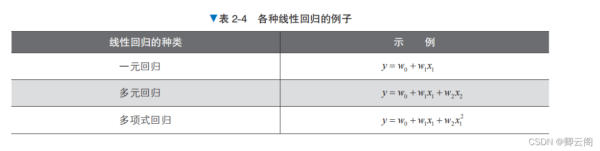
机器学习-算法 1:线性回归
🌞欢迎来到机器学习的世界🌈博客主页:卿云阁💌欢迎关注🎉点赞👍收藏⭐️留言📝🌟本文由卿云阁原创!🌠本阶段属于练气阶段,希望各位仙友顺利完成突破📆首发时间:🌹2021年3月19日🌹✉️希望可以和大家一起完成进阶之路!🙏作者水平很有限,如果发现错误,请留言轰炸哦!万分感谢!🍈 一、应用最小二乘法的简单线性回归import numpy as npimport matplotlib
🌞欢迎来到机器学习的世界
🌈博客主页:卿云阁💌欢迎关注🎉点赞👍收藏⭐️留言📝
🌟本文由卿云阁原创!
🌠本阶段属于练气阶段,希望各位仙友顺利完成突破
📆首发时间:🌹2021年3月19日🌹
✉️希望可以和大家一起完成进阶之路!
🙏作者水平很有限,如果发现错误,请留言轰炸哦!万分感谢!
目录
🍉二. 应用polyfit实现最小二乘法的线性回归和相关性R计算

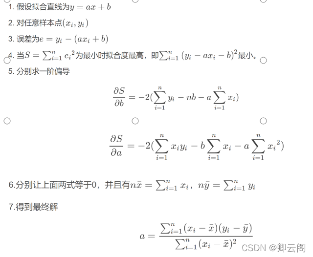
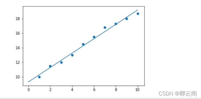
🍈 一、应用最小二乘法的简单线性回归
import numpy as np
import matplotlib.pyplot as plt

def calcAB(x,y):
    n = len(x)
    sumX,sumY,sumXY,sumXX =0,0,0,0
    for i in range(0,n):
        sumX  += x[i]
        sumY  += y[i]
        sumXX += x[i]*x[i]
        sumXY += x[i]*y[i]
    a = (n*sumXY -sumX*sumY)/(n*sumXX -sumX*sumX)
    b = (sumXX*sumY - sumX*sumXY)/(n*sumXX-sumX*sumX)
    return a,b,
xi = [1,2,3,4,5,6,7,8,9,10]
yi = [10,11.5,12,13,14.5,15.5,16.8,17.3,18,18.7]
a,b=calcAB(xi,yi)
print("y = %10.5fx + %10.5f" %(a,b))
x = np.linspace(0,10)  #指定的间隔内返回均匀间隔的数字
y = a * x + b
plt.plot(x,y)
plt.scatter(xi,yi)
plt.show()
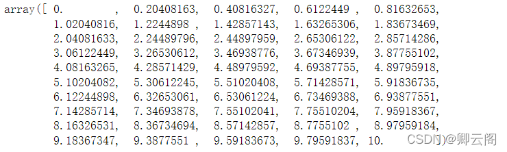
1.np.linspace
通过定义均匀间隔创建数值序列。其实,需要指定间隔起始点、终止端,以及指定分隔值总数(包括起始点和终止点);最终函数返回间隔类均匀分布的数值序列。请看示例:
np.linspace(start = 0, stop = 100, num = 5)
代码生成 NumPy 数组 (ndarray 对象),结果如下:array([ 0., 25., 50., 75., 100.])num (可选)
num 参数控制结果中共有多少个元素。如果num=5,则输出数组个数为5.该参数可选,缺省为50.
图片选自:https://blog.csdn.net/neweastsun/article/details/9967602
import numpy as np
x = np.linspace(0,10)
x
🍉二. 应用polyfit实现最小二乘法的线性回归和相关性R计算
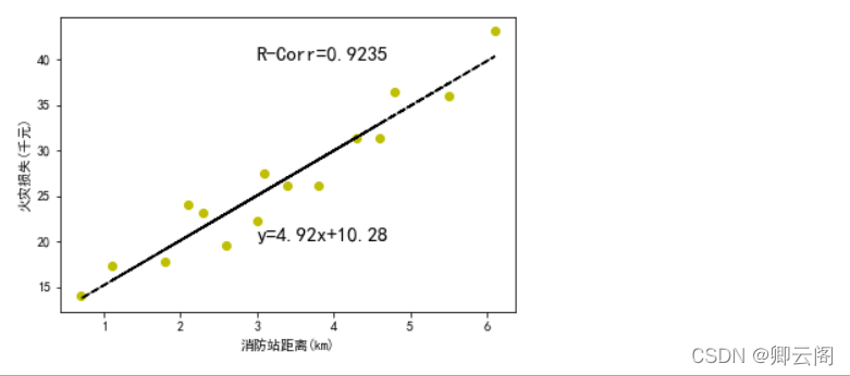
## 火灾损失表
### 距离消防站km
x = [3.4, 1.8, 4.6, 2.3, 3.1, 5.5, 0.7, 3.0, 2.6, 4.3, 2.1, 1.1, 6.1, 4.8, 3.8]
### 火灾损失 千元
y = [26.2, 17.8, 31.3, 23.1, 27.5, 36.0, 14.1, 22.3, 19.6, 31.3, 24.0, 17.3, 43.2, 36.4, 26.1]
import matplotlib
from matplotlib import pyplot as plt
import numpy as np
import math
## 解决中文字符显示不全
from matplotlib.font_manager import FontProperties
font = FontProperties(fname=r"c:\windows\fonts\simsun.ttc", size=12)  #使用指定字体路径和内置字体名称初始化
matplotlib.rcParams['font.sans-serif'] = ['SimHei']     #用来显示中文标签
matplotlib.rcParams['axes.unicode_minus']=False      #用来显示负号
fit = np.polyfit(x, y, 1)
fit_fn = np.poly1d(fit)

def computeCorrelation(X, Y):
    xBar = np.mean(X)     #求x的平均数
    yBar = np.mean(Y)     #求y的平均数
    SSR = 0
    varX = 0
    varY = 0
    for i in range(0 , len(X)):
        diffXXBar = X[i] - xBar
        diffYYBar = Y[i] - yBar
        SSR += (diffXXBar * diffYYBar)
        varX +=  diffXXBar**2 #x的方差
        varY += diffYYBar**2   #y的方差
    SST = math.sqrt(varX * varY)
    return (SSR / SST)**2     #相关性的计算
r2=computeCorrelation(x,y)
plt.plot(x, y, 'yo', x, fit_fn(x), '--k') #'yo'表示用黄色的实心圈,'--k'表示黑色破折线
plt.xlabel('消防站距离(km)')
plt.ylabel('火灾损失(千元)')
plt.annotate('y={:.2f}x+{:.2f}'.format(fit[0],fit[1]), xy=(3,20), fontsize=15)
plt.annotate('R-Corr={:.4f}'.format(r2),xy=(3,40),fontsize=15) #fontsize字体尺寸
plt.show()
通过数据,我们不难发现距离消防站越近,损失越小。
plt.rcParams参数设置
https://blog.csdn.net/Spratumn/article/details/100625967?ops_request_misc=%257B%2522request%255Fid%2522%253A%2522164775972816780261917137%2522%252C%2522scm%2522%253A%252220140713.130102334.pc%255Fall.%2522%257D&request_id=164775972816780261917137&biz_id=0&utm_medium=distribute.pc_search_result.none-task-blog-2~all~first_rank_ecpm_v1~rank_v31_ecpm-2-100625967.142%5Ev2%5Epc_search_result_cache,143%5Ev4%5Econtrol&utm_term=matplotlib.rcParams%5Bfont.sans-serif%5D+%3D+%5BSimHei%5D&spm=1018.2226.3001.4187拟合方法之np.polyfit、np.poly1d
Matplotlib库学习(一)plt.plot
import numpy as np
### 距离消防站km
x = [3.4, 1.8, 4.6, 2.3, 3.1, 5.5, 0.7, 3.0, 2.6, 4.3, 2.1, 1.1, 6.1, 4.8, 3.8]
### 火灾损失 千元
y = [26.2, 17.8, 31.3, 23.1, 27.5, 36.0, 14.1, 22.3, 19.6, 31.3, 24.0, 17.3, 43.2, 36.4, 26.1]
fit = np.polyfit(x, y, 1)
fit

结果:
array([ 4.91933073, 10.27792855])
即:4.91933073为x 的系数,10.27792855为常数项
import numpy as np ### 距离消防站km x = [3.4, 1.8, 4.6, 2.3, 3.1, 5.5, 0.7, 3.0, 2.6, 4.3, 2.1, 1.1, 6.1, 4.8, 3.8] ### 火灾损失 千元 y = [26.2, 17.8, 31.3, 23.1, 27.5, 36.0, 14.1, 22.3, 19.6, 31.3, 24.0, 17.3, 43.2, 36.4, 26.1] fit = np.polyfit(x, y, 1) fit_fn = np.poly1d(fit) #根据系数构造多项式 print(fit_fn) 结果: 4.919 x + 10.28
🍊三, 基于LinearRegression实现最小二乘法线性回归及回归评价指标
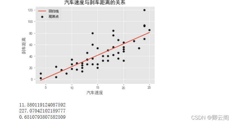
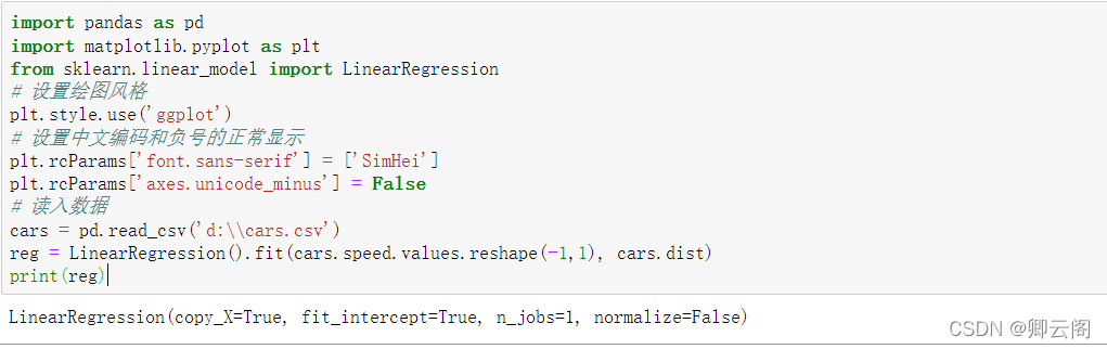
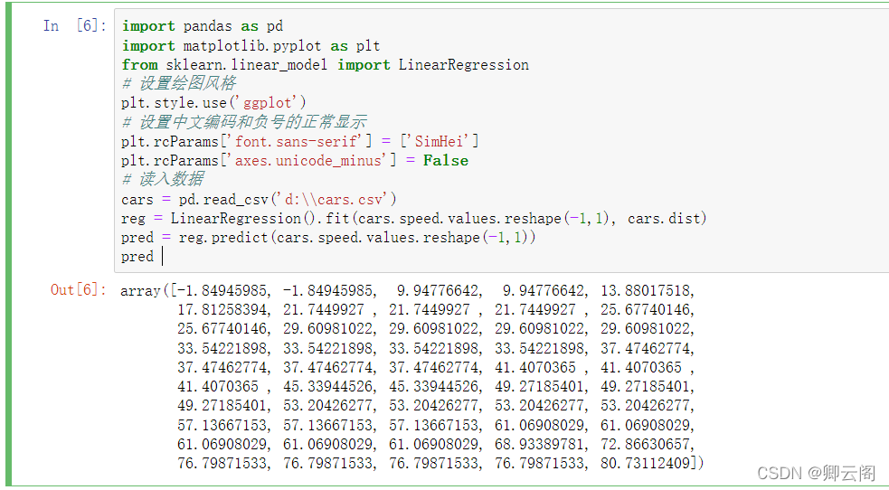
import pandas as pd
import matplotlib.pyplot as plt
from sklearn.linear_model import LinearRegression
# 设置绘图风格
plt.style.use('ggplot')
# 设置中文编码和负号的正常显示
plt.rcParams['font.sans-serif'] = ['SimHei']
plt.rcParams['axes.unicode_minus'] = False
# 读入数据
cars = pd.read_csv('d:\\cars.csv')
# 散点图
plt.scatter(cars.speed, # x轴数据为汽车速度
            cars.dist, # y轴数据为汽车的刹车距离
            s = 30, # 设置点的大小
            c = 'black', # 设置点的颜色
            marker = 'o', # 设置点的形状
            alpha = 0.9, # 设置点的透明度
            linewidths = 0.3, # 设置散点边界的粗细
            label = '观测点'
            )
# 建模
reg = LinearRegression().fit(cars.speed.values.reshape(-1,1), cars.dist)
# 回归预测值
pred = reg.predict(cars.speed.values.reshape(-1,1))
# 绘制回归线
plt.plot(cars.speed, pred, linewidth = 2, label = '回归线')
# 添加轴标签和标题
plt.title('汽车速度与刹车距离的关系')
plt.xlabel('汽车速度')
plt.ylabel('刹车距离')
# 去除图边框的顶部刻度和右边刻度
plt.tick_params(top = 'off', right = 'off')
# 显示图例
plt.legend(loc = 'upper left')
# 显示图形
plt.show()
# 模型评价:
from sklearn.metrics import mean_absolute_error# """计算y_true和y_predict之间的RMSE"""
print(mean_absolute_error(cars.dist, pred))
from sklearn.metrics import mean_squared_error# """计算y_true和y_predict之间的MSE"""
print(mean_squared_error(cars.dist, pred))
from sklearn.metrics import r2_score #"""计算y_true和y_predict之间的R Square"""
print(r2_score(cars.dist, pred))
Python函数reshape(-1,1)到底有什么用?
机器学习之线性回归 Linear Regression(二)Python实现
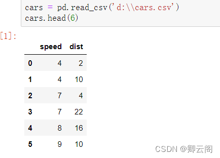
读取前六行的数据
建模
LinearRegression(fit_intercept=True,normalize=False,copy_X=True,n_jobs=1)

fit_intercept:是否有截据,如果没有则直线过原点。

normalize:是否将数据归一化。

copy_X:默认为True,当为True时,X会被copied,否则X将会被覆写。

n_jobs:默认值为1。计算时使用的核数
回归预测值
🍅四,基于tensorflow 2.0实现线性拟合
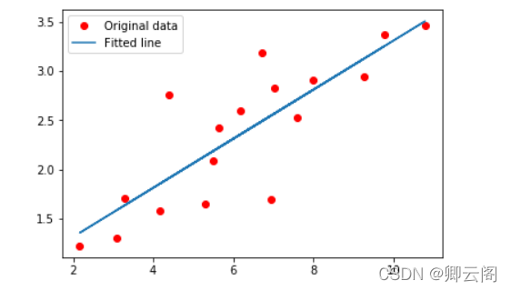
#tensorflow 2.0实现线性拟合
import tensorflow as tf
import numpy as np
from matplotlib import pyplot as plt

# 一些参数
learning_rate = 0.01  # 学习率
training_steps = 2000  # 训练次数
display_step = 50  # 训练50次输出一次

# 训练数据
X = np.array([3.3,4.4,5.5,6.71,6.93,4.168,9.779,6.182,7.59,2.167,
              7.042,10.791,5.313,7.997,5.654,9.27,3.1])
Y = np.array([1.7,2.76,2.09,3.19,1.694,1.573,3.366,2.596,2.53,1.221,
              2.827,3.465,1.65,2.904,2.42,2.94,1.3])
n_samples = X.shape[0]

# 随机初始化权重和偏置
W = tf.Variable(np.random.randn(), name="weight")
b = tf.Variable(np.random.randn(), name="bias")

# 线性回归函数
def linear_regression(x):
    return W*x + b

# 损失函数
def mean_square(y_pred, y_true):
    return tf.reduce_sum(tf.pow(y_pred-y_true, 2)) / (2 * n_samples)

# 优化器采用随机梯度下降(SGD)
optimizer = tf.optimizers.SGD(learning_rate)

# 计算梯度,更新参数
def run_optimization():
    # tf.GradientTape()梯度带,可以查看每一次epoch的参数值
    with tf.GradientTape() as g:
        pred = linear_regression(X)
        loss = mean_square(pred, Y)
    # 计算梯度
    gradients = g.gradient(loss, [W, b])
    # 更新W,b
    optimizer.apply_gradients(zip(gradients, [W, b]))

# 开始训练
for step in range(1, training_steps+1):
    run_optimization()
    if step % display_step == 0:
        pred = linear_regression(X)
        loss = mean_square(pred, Y)
        print("step: %i, loss: %f, W: %f, b: %f" % (step, loss, W.numpy(), b.numpy()))

plt.plot(X, Y, 'ro', label='Original data')
plt.plot(X, np.array(W * X + b), label='Fitted line')
plt.legend()
plt.show()
结果: step: 50, loss: 0.078285, W: 0.230760, b: 0.946792 step: 100, loss: 0.078129, W: 0.231990, b: 0.938072 step: 150, loss: 0.077992, W: 0.233148, b: 0.929866 step: 200, loss: 0.077871, W: 0.234237, b: 0.922144 step: 250, loss: 0.077763, W: 0.235262, b: 0.914876 step: 300, loss: 0.077667, W: 0.236227, b: 0.908037 step: 350, loss: 0.077583, W: 0.237135, b: 0.901600 step: 400, loss: 0.077508, W: 0.237989, b: 0.895543 step: 450, loss: 0.077442, W: 0.238793, b: 0.889843 step: 500, loss: 0.077383, W: 0.239550, b: 0.884479 step: 550, loss: 0.077331, W: 0.240262, b: 0.879431 step: 600, loss: 0.077285, W: 0.240932, b: 0.874680 step: 650, loss: 0.077244, W: 0.241563, b: 0.870209 step: 700, loss: 0.077208, W: 0.242156, b: 0.866002 step: 750, loss: 0.077176, W: 0.242715, b: 0.862042 step: 800, loss: 0.077148, W: 0.243240, b: 0.858316 step: 850, loss: 0.077123, W: 0.243735, b: 0.854809 step: 900, loss: 0.077101, W: 0.244200, b: 0.851509 step: 950, loss: 0.077081, W: 0.244638, b: 0.848404 step: 1000, loss: 0.077064, W: 0.245051, b: 0.845481 step: 1050, loss: 0.077048, W: 0.245439, b: 0.842731 step: 1100, loss: 0.077035, W: 0.245804, b: 0.840142 step: 1150, loss: 0.077023, W: 0.246147, b: 0.837706 step: 1200, loss: 0.077012, W: 0.246471, b: 0.835414 step: 1250, loss: 0.077002, W: 0.246775, b: 0.833256 step: 1300, loss: 0.076994, W: 0.247061, b: 0.831226 step: 1350, loss: 0.076986, W: 0.247331, b: 0.829316 step: 1400, loss: 0.076980, W: 0.247584, b: 0.827518 step: 1450, loss: 0.076974, W: 0.247823, b: 0.825826 step: 1500, loss: 0.076969, W: 0.248048, b: 0.824233 step: 1550, loss: 0.076964, W: 0.248259, b: 0.822735 step: 1600, loss: 0.076960, W: 0.248458, b: 0.821325 step: 1650, loss: 0.076957, W: 0.248645, b: 0.819998 step: 1700, loss: 0.076953, W: 0.248821, b: 0.818749 step: 1750, loss: 0.076951, W: 0.248987, b: 0.817573 step: 1800, loss: 0.076948, W: 0.249143, b: 0.816467 step: 1850, loss: 0.076946, W: 0.249290, b: 0.815426 step: 1900, loss: 0.076944, W: 0.249428, b: 0.814447 step: 1950, loss: 0.076942, W: 0.249558, b: 0.813525 step: 2000, loss: 0.076941, W: 0.249680, b: 0.81265


魔乐社区(Modelers.cn) 是一个中立、公益的人工智能社区,提供人工智能工具、模型、数据的托管、展示与应用协同服务,为人工智能开发及爱好者搭建开放的学习交流平台。社区通过理事会方式运作,由全产业链共同建设、共同运营、共同享有,推动国产AI生态繁荣发展。
更多推荐


 0
0 0
0- 0


 已为社区贡献9条内容

所有评论(0)