阅读前可参考NumPy文章

https://blog.csdn.net/MinggeQingchun/article/details/148253682https://blog.csdn.net/MinggeQingchun/article/details/148253682‌SciPy‌ 是一个基于NumPy的开源Python库，专为科学计算设计，提供了大量高效算法和工具集，涵盖数学、物理、工程等领域的关键问题。

一、SciPy 基础结构

1、SciPy核心功能

1、线性代数：通过scipy.linalg提供矩阵运算（如LU分解，特征值计算）、线性方程组求解

2、优化算法：scipy.optimize支持无约束（如BFGS）和有约束优化（如线性约束），适用于最小化目标函数或解决复杂优化问题

3、数值积分与微分方程：scipy.integrate模块可进行定积分计算和常/偏微分方程求解（如阻尼器震荡的数值模拟）

4、信号处理：scipy.signal提供滤波器设计（如低通滤波器）、傅里叶变换工具，适用于音频或图像处理场景

5、统计与特殊函数：scipy.stats和scipy.special包含概率分布计算、贝叶斯统计以及特殊数学函数（如伽玛函数）等

2、SciPy底层实现原理以及高效性能

SciPy 的核心算法采用 C/Fortran/C++ 编写，结合 Python 的灵活性和 NumPy 的数组操作能力，实现高性能计算。如：

【1】稀疏矩阵支持（如 scipy.sparse），适用于大规模数据处理

【2】多线程优化（例如积分模块的并行计算），提升大规模运算效率。‌‌

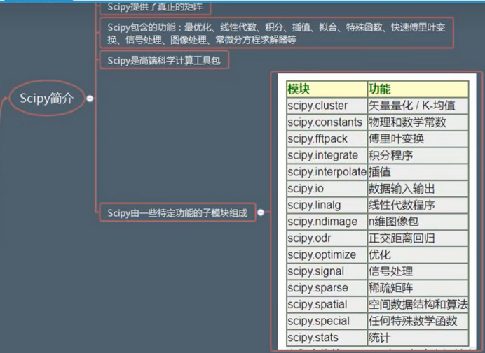
SciPy 由多个子模块组成，每个子模块专注于特定领域的科学计算：

import scipy
from scipy import optimize, integrate, interpolate, linalg, stats, fft, signal, ndimage, sparse

二、主要功能模块

2.1 优化与求根 (scipy.optimize)

1、最小化函数：

from scipy.optimize import minimize

def rosen(x):
    return sum(100.0*(x[1:]-x[:-1]**2.0)**2.0 + (1-x[:-1])**2.0)

x0 = [1.3, 0.7, 0.8, 1.9, 1.2]
res = minimize(rosen, x0, method='nelder-mead', options={'xatol': 1e-8, 'disp': True})
print(res.x)

2、方程求根：

from scipy.optimize import root

def func(x):
    return x + 2*np.cos(x)

sol = root(func, 0.3)
print(sol.x)

2.2 积分 (scipy.integrate)

定积分计算：

from scipy.integrate import quad

result, error = quad(lambda x: np.exp(-x**2), -np.inf, np.inf)
print(f"积分结果: {result}, 误差估计: {error}")

常微分方程求解：

from scipy.integrate import solve_ivp

def lotkavolterra(t, z, a, b, c, d):
    x, y = z
    return [a*x - b*x*y, -c*y + d*x*y]

sol = solve_ivp(lotkavolterra, [0, 15], [10, 5], args=(1.5, 1, 3, 1), dense_output=True)

2.3 插值 (scipy.interpolate)

一维插值：

from scipy.interpolate import interp1d

x = np.linspace(0, 10, num=11)
y = np.cos(-x**2/9.0)
f = interp1d(x, y, kind='cubic')

xnew = np.linspace(0, 10, num=41)
plt.plot(x, y, 'o', xnew, f(xnew), '-')
plt.legend(['数据点', '三次样条'], loc='best')
plt.show()

2.4 线性代数 (scipy.linalg)

矩阵运算：

from scipy import linalg

A = np.array([[1, 2], [3, 4]])
# 计算行列式
print(linalg.det(A))
# 计算逆矩阵
print(linalg.inv(A))
# 特征值和特征向量
eigenvalues, eigenvectors = linalg.eig(A)

2.5 统计函数 (scipy.stats)

1、概率分布：

from scipy import stats

# 正态分布
norm_dist = stats.norm(loc=0, scale=1)
print(f"PDF at 0: {norm_dist.pdf(0)}")
print(f"CDF at 1: {norm_dist.cdf(1)}")

# 生成随机变量
samples = norm_dist.rvs(size=1000)
plt.hist(samples, bins=30, density=True)
x = np.linspace(-4, 4, 100)
plt.plot(x, norm_dist.pdf(x))
plt.show()

2、假设检验：

# t检验
a = np.random.normal(0, 1, size=100)
b = np.random.normal(1, 1, size=100)
t_stat, p_val = stats.ttest_ind(a, b)
print(f"t统计量: {t_stat}, p值: {p_val}")

2.6 傅里叶变换 (scipy.fft)

from scipy.fft import fft, fftfreq

# 采样频率
N = 600
T = 1.0 / 800.0
x = np.linspace(0.0, N*T, N, endpoint=False)
y = np.sin(50.0 * 2.0*np.pi*x) + 0.5*np.sin(80.0 * 2.0*np.pi*x)

yf = fft(y)
xf = fftfreq(N, T)[:N//2]

plt.plot(xf, 2.0/N * np.abs(yf[0:N//2]))
plt.grid()
plt.show()

 可参考

深入浅出的讲解傅里叶变换（真正的通俗易懂） - h2z - 博客园

2.7 信号处理 (scipy.signal)

from scipy import signal

# 设计一个低通滤波器
b, a = signal.butter(4, 100, 'low', analog=True)
w, h = signal.freqs(b, a)
plt.semilogx(w, 20*np.log10(abs(h)))
plt.title('Butterworth滤波器频率响应')
plt.xlabel('频率 [rad/s]')
plt.ylabel('振幅 [dB]')
plt.grid(which='both', axis='both')
plt.show()

2.8 图像处理 (scipy.ndimage)

from scipy import ndimage
from scipy import misc

# 图像处理示例
face = misc.face(gray=True)
blurred_face = ndimage.gaussian_filter(face, sigma=3)

fig, (ax1, ax2) = plt.subplots(1, 2, figsize=(10, 5))
ax1.imshow(face, cmap='gray')
ax1.set_title('原始图像')
ax2.imshow(blurred_face, cmap='gray')
ax2.set_title('高斯模糊')
plt.show()

2.9 稀疏矩阵 (scipy.sparse)

from scipy import sparse

# 创建稀疏矩阵
row = np.array([0, 1, 2, 0])
col = np.array([0, 1, 2, 2])
data = np.array([1, 1, 1, 1])
sparse_matrix = sparse.coo_matrix((data, (row, col)), shape=(3, 3))

print("稀疏矩阵:")
print(sparse_matrix.toarray())

3 实际应用

3.1、曲线拟合

from scipy.optimize import curve_fit

def func(x, a, b, c):
    return a * np.exp(-b * x) + c

xdata = np.linspace(0, 4, 50)
y = func(xdata, 2.5, 1.3, 0.5)
ydata = y + 0.2 * np.random.normal(size=len(xdata))

popt, pcov = curve_fit(func, xdata, ydata)
plt.plot(xdata, ydata, 'b-', label='数据')
plt.plot(xdata, func(xdata, *popt), 'r-', label='拟合')
plt.legend()
plt.show()

3.2、数值积分应用

from scipy.integrate import dblquad

# 计算二重积分
def integrand(y, x):
    return np.exp(-x**2 - y**2)

x_lower = 0
x_upper = 10
y_lower = 0
y_upper = 10

result, error = dblquad(integrand, x_lower, x_upper, 
                        lambda x: y_lower, lambda x: y_upper)
print(f"积分结果: {result}, 误差估计: {error}")

性能优化技巧

1. 向量化运算：尽量使用 NumPy/SciPy 的向量化操作代替循环

2. 使用稀疏矩阵：对于大型稀疏矩阵问题

3. 选择合适算法：根据问题特点选择最优的数值方法

4. JIT 编译：结合 Numba 加速关键代码