基于LSTM、GRU、RNN的锂电池数据预处理与时序数据预测
本文基于CALCE电池数据集,采用LSTM、GRU和RNN三种深度学习模型进行电池寿命预测研究。首先对原始数据进行预处理,包括异常值剔除和容量计算。在模型构建方面,对比了单步预测和多步预测两种方法,其中单步预测采用fixed、moving和mobile三种递归策略,多步预测则探讨了不同窗口尺寸(base_num, pre_num)组合对预测精度的影响。
摘要
时序数据预测的深度学习方法主要可以分为单步预测和多步预测。单步预测指的是通过将数据输入训练好的模型一次预测未来一个数据点,如果想要预测未来多个时间点的数据就需要进行递归运算,从而也会导致误差的累计;而多步预测指的是模型一次性预测出未来多个时间点的数据,误差也较小。本文将在对CALCE数据集预处理的基础上利用LSTM、GRU、RNN三种深度学习模型对电池寿命(电池容量,capacity)进行预测。
CALCE数据集预处理
马里兰的数据是多个excel表中存放的,其中CS2电池的数据是采用标准的恒流恒压充电方式,首先用0.5C的电流充电至4.2V,之后按照4.2V恒压充电,直到充电电流降到0.05A,除了特殊情况,电池的放电电流按照1C放电至2.7V。
CS2 电池数据中CS2_n指的是电池编号,下面是具体的一些excel数据的命名规则,以CS2_35为例,CS2 35 2411前面CS2是电池的类型;35表示电池的编号;2411表示电池试验进行的日期。参考如下网址:https://github.com/XiuzeZhou/CALCE/blob/main/RNN%20%26%20LSTM%20-%20CALCE.ipynb
(1)在文件中读取放电阶段的数据(步骤序号为7),主要有:容量,电流和电压
(2)去除异常值
def drop_outlier(array,count,bins):
    index = []
    range_ = np.arange(1,count,bins)
    for i in range_[:-1]:
        array_lim = array[i:i+bins]
        sigma = np.std(array_lim)
        mean = np.mean(array_lim)
        th_max,th_min = mean + sigma*2, mean - sigma*2
        idx = np.where((array_lim < th_max) & (array_lim > th_min))
        idx = idx[0] + i
        index.extend(list(idx))
    return np.array(index)
(3)计算capacity
![]() 是时间t时的瞬时累计容量(单位:安时,Ah)。
是时间t时的瞬时累计容量(单位:安时,Ah)。
![]() 是第
是第![]() 个时间点的电流(单位:安培,A)。
个时间点的电流(单位:安培,A)。
![]() 是第
是第![]() 个时间点与上一个时间点的时间差(单位:秒,s)
个时间点与上一个时间点的时间差(单位:秒,s)
3600是将秒转换为小时的转换因子(1小时=3600秒)
if(len(list(d_c)) != 0):
    time_diff = np.diff(list(d_t))
    d_c = np.array(list(d_c))[1:]
    discharge_capacity = time_diff*d_c/3600 # Q = A*h
    discharge_capacity = [np.sum(discharge_capacity[:n]) for n in range(discharge_capacity.shape[0])]
    discharge_capacities.append(-1*discharge_capacity[-1])

    dec = np.abs(np.array(d_v) - 3.8)[1:]
    start = np.array(discharge_capacity)[np.argmin(dec)]
    dec = np.abs(np.array(d_v) - 3.4)[1:]
    end = np.array(discharge_capacity)[np.argmin(dec)]
    health_indicator.append(-1 * (end - start))

    internal_resistance.append(np.mean(np.array(d_im)))
    count += 1
(4)处理好的数据展示
#Rated_Capacity = 1.1
fig, ax = plt.subplots(1, figsize=(12, 8))
color_list = ['b:', 'g--', 'r-.', 'c.']
for name,color in zip(Battery_list, color_list):
    df_result = Battery[name]
    ax.plot(df_result['cycle'], df_result['capacity'], color, label='Battery_'+name)
ax.set(xlabel='Discharge cycles', ylabel='Capacity (Ah)', title='Capacity degradation at ambient temperature of 1°C')
plt.legend()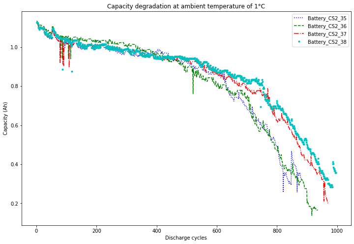
数据标准化
这里之所以不选用最大最小值归一化(MinMaxScaler方法)是因为归一化易受异常值影响(偏离数据曲线较大的值),而标准化由于减去平均值再除以标准差,可以缩小这种影响。标准差可以手动计算也可以调用sklearn库中的StandardScaler方法。
from sklearn.preprocessing import StandardScaler, MinMaxScaler
import numpy as np

# 使用 StandardScaler 进行标准化
scaler = StandardScaler()
standardized_data = scaler.fit_transform(data)
定义模型与数据加载器。
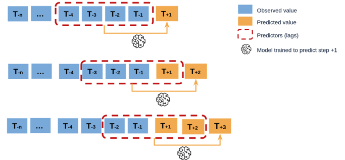
利用深度学习模型训练时序数据,一般是将数据分为一个个滑动窗口,每个窗口就是一个训练样本,窗口大小为base_num+pre_num,其中,前base_num个数据点为训练数据,后pre_num个数据点作为训练标签,训练完成之后,将测试机也处理成窗口的形式,将前面的数据输入模型,输出后面的预测数据和label进行比较,计算误差即可。
对于单步预测,pre_num设置为1,对于多步预测,pre_num设置为想要预测的步数长度。
class MyDataset(Dataset):
    def __init__(self, path):
        data = pd.read_excel(path, header=0)
        self.x = data.values[:, :base_num].astype(np.float32)
        self.y = data.values[:, base_num:].astype(np.float32)
        self.means = []
        self.stds = []

        for i in range(self.x.shape[0]):
            mean = np.mean(self.x[i, :])
            std = np.std(self.x[i, :])
            self.x[i, :] = (self.x[i, :] - mean) / std
            self.y[i, :] = (self.y[i, :] - mean) / std
            self.means.append(mean)
            self.stds.append(std)
        print(np.min(self.stds))
    def __getitem__(self, index):
        return np.expand_dims(self.x[index, :], axis=-1), self.y[index, :]

    def __len__(self):
        return self.x.shape[0]

class MyModel_GRU(nn.Module):
    def __init__(self):
        super().__init__()
        self.gru = nn.GRU(1, base_num, num_layers=1, bias=True, batch_first=True)
        self.linear = nn.Linear(in_features=base_num * base_num, out_features=pre_num)

    def forward(self, x):
        x, hn = self.gru(x)
        x = x.reshape(x.shape[0], -1)
        x = self.linear(x)
        return x

class MyModel_LSTM(nn.Module):
    def __init__(self):
        super().__init__()
        self.lstm = nn.LSTM(1, base_num, num_layers=1, bias=True, batch_first=True)
        self.linear = nn.Linear(in_features=base_num * base_num, out_features=pre_num)

    def forward(self, x):
        x, (hn, cn) = self.lstm(x)
        x = x.reshape(x.shape[0], -1)
        x = self.linear(x)
        return x

class MyModel_RNN(nn.Module):
    def __init__(self):
        super().__init__()
        self.rnn = nn.RNN(1, base_num, num_layers=1, bias=True, batch_first=True)
        self.linear = nn.Linear(in_features=base_num * base_num, out_features=pre_num)

    def forward(self, x):
        x, hn = self.rnn(x)
        x = x.reshape(x.shape[0], -1)
        x = self.linear(x)
        return x
训练模型、打印损失
def train_model(model, train_dataloader, test_dataloader, criterion, optimizer, epochs, patience):
    best_val_loss = float('inf')
    epochs_no_improve = 0

    for epoch in range(epochs):
        model.train()
        for X, y in train_dataloader:
            X, y = X.to(device), y.to(device)
            p = model(X)
            loss = criterion(p, y)
            loss.backward()
            optimizer.step()
            optimizer.zero_grad()

        model.eval()
        train_loss, test_loss = 0, 0
        with torch.no_grad():
            for X, y in train_dataloader:
                X, y = X.to(device), y.to(device)
                p = model(X)
                train_loss += criterion(p, y).item()

            for X, y in test_dataloader:
                X, y = X.to(device), y.to(device)
                p = model(X)
                test_loss += criterion(p, y).item()

        train_loss /= len(train_dataloader)
        test_loss /= len(test_dataloader)
        print(f'Epoch {epoch + 1:2d}: train_loss = {train_loss:.4f}, test_loss = {test_loss:.4f}')

        if test_loss < best_val_loss:
            best_val_loss = test_loss
            epochs_no_improve = 0
            torch.save(model.state_dict(), 'best_model.pth')
        else:
            epochs_no_improve += 1
            if epochs_no_improve >= patience:
                print(f'Early stopping at epoch {epoch + 1}')
                break

    model.load_state_dict(torch.load('best_model.pth'))
    return model
模型评估、绘制图像
def evaluate_model(model, test_dataloader, test_data):
    model.eval()
    predictions, actuals = [], []
    with torch.no_grad():
        for X, y in test_dataloader:
            X = X.to(device)
            p = model(X)
            predictions.append(p.cpu().numpy())
            actuals.append(y.numpy())

    predictions = np.concatenate(predictions)
    actuals = np.concatenate(actuals)

    # 恢复原始数据
    real = actuals[:, -1] * np.array(test_data.stds) + np.array(test_data.means)
    predict = predictions[:, -1] * np.array(test_data.stds) + np.array(test_data.means)

    plt.plot(real, linestyle='-.', color='blue', label='Actual')
    plt.plot(predict, linestyle='--', color='red',label='Predict')
    plt.legend()
    plt.show()
    rmse = np.sqrt(np.mean((np.array(real) - np.array(predict.reshape(-1))) ** 2))
    print(f"RMSE: {rmse}")
LSTM、GRU、RNN图像结果及模型性能指标(RMSE,均方误差)结果见后文对比分析模块
单步递归预测的三种策略(迭代多步)
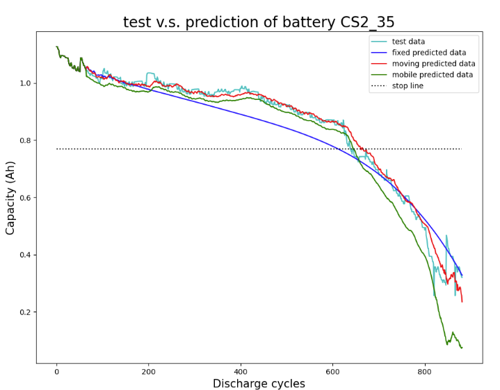
单步预测都是数据经过模型一次只预测未来一个点,若想预测未来一段时间内的数据情况则需要进行递归预测。递归预测大致又分为如下三种模式。
(1)fixed模式
每次预测一个点,将预测到的值加入预测数据末端,窗口后移一步,保证窗口大小与模型输入尺寸一致,一直进行递归,只用初始的pre_num个数据可从头预测到尾,误差累积最大。
# fixed
x = np.reshape(np.array(test_x[-feature_size:])/Rated_Capacity, (-1, feature_num, feature_size)).astype(np.float32)
x = torch.from_numpy(x).to(device)
x = x.repeat(1, K, 1)
pred, _ = model(x)
next_point = pred.data.cpu().numpy()[0,0] * Rated_Capacity
test_x.append(next_point)      # The test values are added to the original sequence to continue to predict the next point
fixed_point_list.append(next_point) # Saves the predicted value of the last point in the output sequence
(2)moving模式
每次预测未来一个数据点,若想预测下一个时间步的数据,需要在模型输入数据的末尾加入新观测到的实际值,类似于在线学习的过程,虽然误差小,但是只能预测未来一步的数据,无法做到对电池寿命提前预警的功能。
# moving
x = np.reshape(np.array(test_sequence[t:t+feature_size])/Rated_Capacity, (-1, 1, feature_size)).astype(np.float32)
x = torch.from_numpy(x).to(device)
x = x.repeat(1, K, 1)
pred, _ = model(x)
next_point = pred.data.cpu().numpy()[0,0] * Rated_Capacity
moving_point_list.append(next_point) # Saves the predicted value of the last point in the output sequence
(3)mobile模式
结合(1)、(2)两种模式,在每个时间点的模型输入末端加上新观测到的数据,窗口滑动一步,并递归预测未来pre_num个数据点。可以去这些数据点的均值或末尾值作为预测到的数据以提前预警(具体选取方式根据具体任务可以修改)。这种方式结合了前两种方法的优势,但仍存在误差累积的缺点(后续实验结果很好地说明了这点)。
# mobile
z = np.reshape(np.array(test_sequence[t:t+feature_size])/Rated_Capacity, (1, 1, feature_size)).astype(np.float32)
for i in range(50):
    z_tensor = torch.from_numpy(z).to(device)
    z_tensor = z_tensor.repeat(1, K, 1)
    predict, _ = model(z_tensor)
    next_point = predict.data.cpu().numpy()[0,0]  # 这里已经是归一化的
    #print(f"Next point for mobile prediction (iteration {i}): {next_point}")
    z = np.concatenate([z[:, :, 1:], np.array(next_point).reshape(1, 1, 1)], axis=2)
# 还原容量
mobile_point_list.append(next_point * Rated_Capacity)
三种模式预测结果对比:
实验结果展示
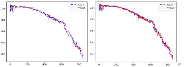
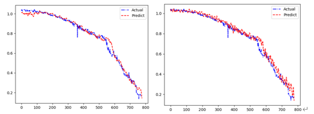
对于单步预测,本实验选择mobile模式在LSTM网络的基础上进行递归预测;对于多步预测,本实验尝试了不同的base_num与pre_num大小的组合例如(63,16)、(128,32)、(256、64)、(256、128)。实验结果显示,多步预测误差比单步预测效果较好(训练成本也略大),并且对于多步预测,base_num至少为pre_num的两倍预测效果才能较好,且随着窗口长度的增加,预测误差也越来越大,因此可以推断,基于Transformer的长距离依赖的模型例如PatchTST、Informer、UniTST或者Conformer可能预测效果会更好(其需要的训练数据更多、训练成本也更大)。
(1)(64,16)左边为LSTM多步预测,右边为单步递归
(2)(128,32)左边为LSTM多步预测,右边为单步递归
(3)(256,64)左边为LSTM多步预测,右边为单步递归
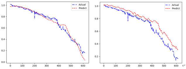
(4)三种模型多步预测与单步预测mobile模式实验结果
|
Model |
(base_num,pre_num) |
Train-loss |
Test-loss |
Predict-RMSE |
|
LSTM |
64,16 |
0.0326 |
0.0238 |
0.029138 |
|
128,32 |
0.4956 |
0.7257 |
0.031113 |
|
|
256,64 |
0.3597 |
0.3770 |
0.047948 |
|
|
256,128 |
0.9026 |
0.8235 |
0.066543 |
|
|
GRU |
64,16 |
0.0319 |
0.0239 |
0.028965 |
|
128,32 |
0.6953 |
0.7934 |
0.031417 |
|
|
256,64 |
0.3574 |
0.3840 |
0.047582 |
|
|
256,128 |
0.8700 |
0.8490 |
0.067261 |
|
|
RNN |
64,16 |
0.0320 |
0.0238 |
0.02924 |
|
128,32 |
0.9337 |
0.7489 |
0.031733 |
|
|
256,64 |
0.3413 |
0.3873 |
0.045177 |
|
|
256,128 |
1.0593 |
1.2217 |
0.061741 |
|
|
LSTM-Mobile |
64,16 |
0.0055 |
0.0073 |
0.027386 |
|
128,32 |
0.0040 |
0.0046 |
0.038160 |
|
|
256,64 |
0.0019 |
0.0022 |
0.093274 |

魔乐社区(Modelers.cn) 是一个中立、公益的人工智能社区,提供人工智能工具、模型、数据的托管、展示与应用协同服务,为人工智能开发及爱好者搭建开放的学习交流平台。社区通过理事会方式运作,由全产业链共同建设、共同运营、共同享有,推动国产AI生态繁荣发展。
更多推荐
 25
25 0
0- 0


 已为社区贡献1条内容

所有评论(0)