一、数据集介绍

MINST数据集分类

1.MNIST数据集

MNIST数据集官网

下载下来的数据集被分成两部分：60000行的训练数据集（mnist.train）和10000行的测试数据集（mnise.test）

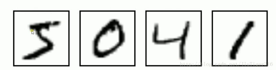
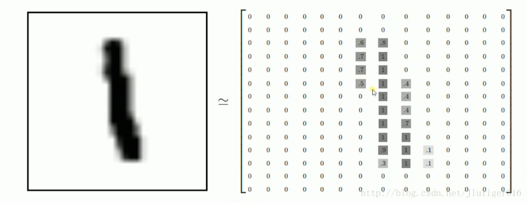
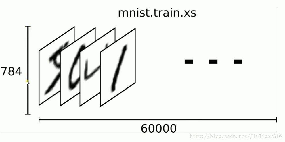
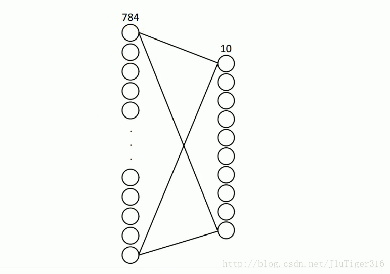
每一张图片包含28*28个像素，我们把这一个数组展开成一个向量，长度是28*28=784。因此在MNIST训练数据集中mnist.train.images是一个形状为[60000，784]的张量，第一个维度数字用来索引图片，第二个维度数字用来索引每张图片的像素点。图片里的某个像素的强度值介于0-1之间。

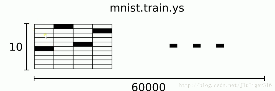
MNIST数据集的标签是介于0-9的数字，我们要把标签转化为“one-hot- vectors”。一个one-hot向量除了某一位数字是1以外，其余维度数字都是0，比如标签0将表示为（[1,0,0,0,0,0,0,0,0,0]）,标签3将表示为（[0,0,0,1,0,0,0,0,0,0]）。
因此，minst.train.labels是一个[60000，10]的数字矩阵。

 

 

传统神经网络存在的问题：

1.权值太多，计算量太大。 
2.权值太多，需要大量样本进行训练。

说明：.一般来说，样本的大小，最好是未知数（权值）的5-30倍

---

局部感受野：

1962年哈佛医学院神经生理学家Hubel和Wiesel通过对猫视觉皮层细胞的研究，提出了感受野（receptive field）的概念，1984年日本学者Fukushima基于感受野概念提出的神经认知机（neocognitron）可以看作是卷积神经网络的第一个实现网络，也是感受野概念在人工神经网络领域的首次应用。

卷积神经网络CNN：

CNN通过感受野和权值共享减少了神经网络需要训练的参数个数。

---

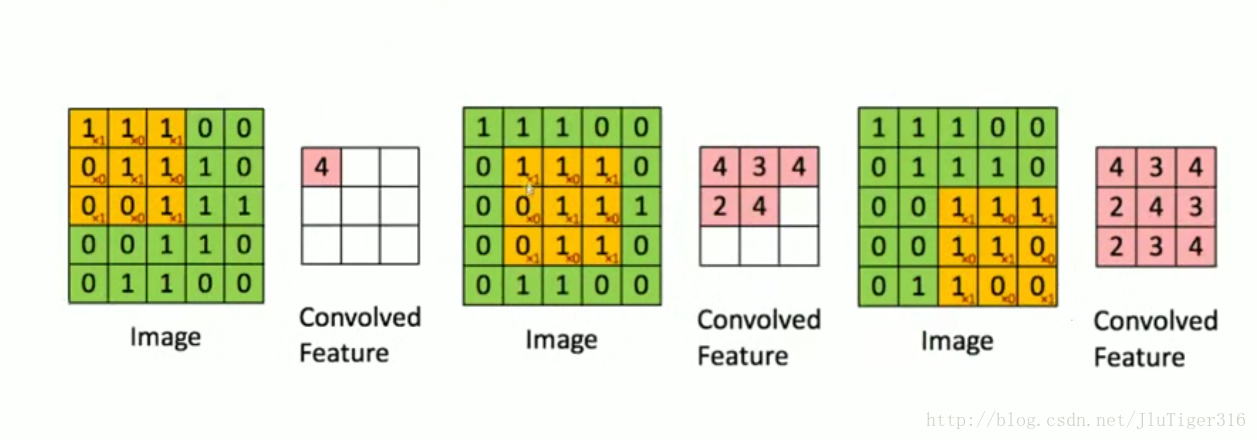
卷积：

     卷积核相当于一个滤波器，不同的卷积核可以对不同的特征进行采样（过滤）

---

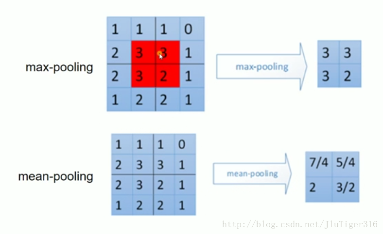
池化 ：

       窗口中的最大值或者平均值

---

对于卷积操作：

SAME PADDING： 给平面外部补0，卷积窗口采样后得到一个跟原来平面大小相同的平面。 
VALID PADDING： 不会超出平面外部，卷积窗口采样后得到一个比原来平面小的平面。

---

对于池化操作：

SAME PADDING： 可能会给平面外部补0。 
VALID PADDING： 不会超出平面外部。

假如有一个28*28的平面，用2*2并且步长为2的窗口对其进行pooling操作 
使用SAME PADDING的方式，得到14*14的平面 
使用VALID PADDING的方式，得到14*14的平面 
假如有一个2*3的平面，用2*2并且步长为2的窗口对其进行pooling操作 
使用SAME PADDING的方式，得到1*2的平面 
使用VALID PADDING的方式，得到1*1的平面

---

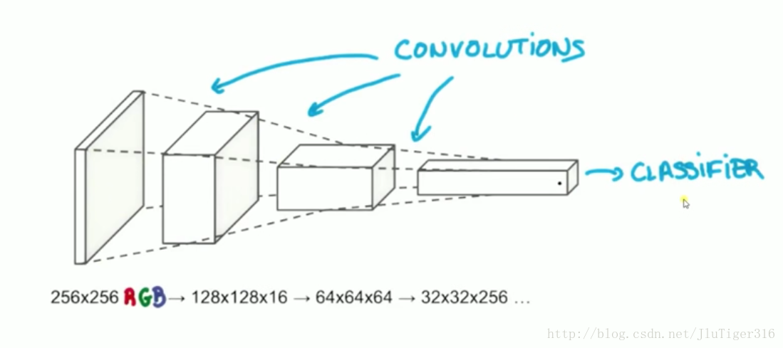
CNN结构：

---

---

 

一.采用简单线性回归进行手写数字分类。

网络结构：

# coding: utf-8

# In[2]:

import tensorflow as tf
from tensorflow.examples.tutorials.mnist import input_data


# In[3]:

#载入数据集
mnist = input_data.read_data_sets("MNIST_data",one_hot=True)

#每个批次的大小
batch_size = 100
#计算一共有多少个批次
n_batch = mnist.train.num_examples // batch_size

#定义两个placeholder
x = tf.placeholder(tf.float32,[None,784])
y = tf.placeholder(tf.float32,[None,10])

#创建一个简单的神经网络
W = tf.Variable(tf.zeros([784,10]))
b = tf.Variable(tf.zeros([10]))
prediction = tf.nn.softmax(tf.matmul(x,W)+b)

#二次代价函数
loss = tf.reduce_mean(tf.square(y-prediction))
#使用梯度下降法
train_step = tf.train.GradientDescentOptimizer(0.2).minimize(loss)

#初始化变量
init = tf.global_variables_initializer()

#结果存放在一个布尔型列表中
correct_prediction = tf.equal(tf.argmax(y,1),tf.argmax(prediction,1))#argmax返回一维张量中最大的值所在的位置
#求准确率
accuracy = tf.reduce_mean(tf.cast(correct_prediction,tf.float32))

with tf.Session() as sess:
    sess.run(init)
    for epoch in range(21):
        for batch in range(n_batch):
            batch_xs,batch_ys =  mnist.train.next_batch(batch_size)
            sess.run(train_step,feed_dict={x:batch_xs,y:batch_ys})
        
        acc = sess.run(accuracy,feed_dict={x:mnist.test.images,y:mnist.test.labels})
        print("Iter " + str(epoch) + ",Testing Accuracy " + str(acc))


# In[ ]:

测试结果：

Extracting MNIST_data\train-images-idx3-ubyte.gz
Extracting MNIST_data\train-labels-idx1-ubyte.gz
Extracting MNIST_data\t10k-images-idx3-ubyte.gz
Extracting MNIST_data\t10k-labels-idx1-ubyte.gz
Iter 0,Testing Accuracy 0.8304
Iter 1,Testing Accuracy 0.8708
Iter 2,Testing Accuracy 0.8808
Iter 3,Testing Accuracy 0.8878
Iter 4,Testing Accuracy 0.8942
Iter 5,Testing Accuracy 0.8967
Iter 6,Testing Accuracy 0.8996
Iter 7,Testing Accuracy 0.902
Iter 8,Testing Accuracy 0.9037
Iter 9,Testing Accuracy 0.9055
Iter 10,Testing Accuracy 0.907
Iter 11,Testing Accuracy 0.9074
Iter 12,Testing Accuracy 0.9073
Iter 13,Testing Accuracy 0.9084
Iter 14,Testing Accuracy 0.9102
Iter 15,Testing Accuracy 0.9112
Iter 16,Testing Accuracy 0.9119
Iter 17,Testing Accuracy 0.912
Iter 18,Testing Accuracy 0.9131
Iter 19,Testing Accuracy 0.9125
Iter 20,Testing Accuracy 0.9134

对如上代码进行优化：

 优化方案两个方向：1.改变batch_size，即每批次的大小。2.增加隐藏层，隐藏层神经元的个数。3.隐藏层之间的激活函数可以用双曲正切函数等。4.权值和偏置值都都需要初始化，初始化的方式。5代价函数，例如可以更改为交叉熵等。6.优化方式，这里用的梯度下降法，或者改变学习率等。7.训练的次数，可以尝试训练更多的次数。

二：采用CNN进行minist手写数字识别

# coding: utf-8

# In[1]:

import tensorflow as tf
from tensorflow.examples.tutorials.mnist import input_data


# In[2]:

mnist = input_data.read_data_sets('MNIST_data',one_hot=True)

#每个批次的大小
batch_size = 100
#计算一共有多少个批次
n_batch = mnist.train.num_examples // batch_size

#参数概要
def variable_summaries(var):
    with tf.name_scope('summaries'):
        mean = tf.reduce_mean(var)
        tf.summary.scalar('mean', mean)#平均值
        with tf.name_scope('stddev'):
            stddev = tf.sqrt(tf.reduce_mean(tf.square(var - mean)))
        tf.summary.scalar('stddev', stddev)#标准差
        tf.summary.scalar('max', tf.reduce_max(var))#最大值
        tf.summary.scalar('min', tf.reduce_min(var))#最小值
        tf.summary.histogram('histogram', var)#直方图

#初始化权值
def weight_variable(shape,name):
    initial = tf.truncated_normal(shape,stddev=0.1)#生成一个截断的正态分布
    return tf.Variable(initial,name=name)

#初始化偏置
def bias_variable(shape,name):
    initial = tf.constant(0.1,shape=shape)
    return tf.Variable(initial,name=name)

#卷积层
def conv2d(x,W):
    #x input tensor of shape `[batch, in_height, in_width, in_channels]`
    #W filter / kernel tensor of shape [filter_height, filter_width, in_channels, out_channels]
    #`strides[0] = strides[3] = 1`. strides[1]代表x方向的步长，strides[2]代表y方向的步长
    #padding: A `string` from: `"SAME", "VALID"`
    return tf.nn.conv2d(x,W,strides=[1,1,1,1],padding='SAME')

#池化层
def max_pool_2x2(x):
    #ksize [1,x,y,1]
    return tf.nn.max_pool(x,ksize=[1,2,2,1],strides=[1,2,2,1],padding='SAME')

#命名空间
with tf.name_scope('input'):
    #定义两个placeholder
    x = tf.placeholder(tf.float32,[None,784],name='x-input')
    y = tf.placeholder(tf.float32,[None,10],name='y-input')
    with tf.name_scope('x_image'):
        #改变x的格式转为4D的向量[batch, in_height, in_width, in_channels]`
        x_image = tf.reshape(x,[-1,28,28,1],name='x_image')


with tf.name_scope('Conv1'):
    #初始化第一个卷积层的权值和偏置
    with tf.name_scope('W_conv1'):
        W_conv1 = weight_variable([5,5,1,32],name='W_conv1')#5*5的采样窗口，32个卷积核从1个平面抽取特征
    with tf.name_scope('b_conv1'):  
        b_conv1 = bias_variable([32],name='b_conv1')#每一个卷积核一个偏置值

    #把x_image和权值向量进行卷积，再加上偏置值，然后应用于relu激活函数
    with tf.name_scope('conv2d_1'):
        conv2d_1 = conv2d(x_image,W_conv1) + b_conv1
    with tf.name_scope('relu'):
        h_conv1 = tf.nn.relu(conv2d_1)
    with tf.name_scope('h_pool1'):
        h_pool1 = max_pool_2x2(h_conv1)#进行max-pooling

with tf.name_scope('Conv2'):
    #初始化第二个卷积层的权值和偏置
    with tf.name_scope('W_conv2'):
        W_conv2 = weight_variable([5,5,32,64],name='W_conv2')#5*5的采样窗口，64个卷积核从32个平面抽取特征
    with tf.name_scope('b_conv2'):  
        b_conv2 = bias_variable([64],name='b_conv2')#每一个卷积核一个偏置值

    #把h_pool1和权值向量进行卷积，再加上偏置值，然后应用于relu激活函数
    with tf.name_scope('conv2d_2'):
        conv2d_2 = conv2d(h_pool1,W_conv2) + b_conv2
    with tf.name_scope('relu'):
        h_conv2 = tf.nn.relu(conv2d_2)
    with tf.name_scope('h_pool2'):
        h_pool2 = max_pool_2x2(h_conv2)#进行max-pooling

#28*28的图片第一次卷积后还是28*28，第一次池化后变为14*14
#第二次卷积后为14*14，第二次池化后变为了7*7
#进过上面操作后得到64张7*7的平面

with tf.name_scope('fc1'):
    #初始化第一个全连接层的权值
    with tf.name_scope('W_fc1'):
        W_fc1 = weight_variable([7*7*64,1024],name='W_fc1')#上一场有7*7*64个神经元，全连接层有1024个神经元
    with tf.name_scope('b_fc1'):
        b_fc1 = bias_variable([1024],name='b_fc1')#1024个节点

    #把池化层2的输出扁平化为1维
    with tf.name_scope('h_pool2_flat'):
        h_pool2_flat = tf.reshape(h_pool2,[-1,7*7*64],name='h_pool2_flat')
    #求第一个全连接层的输出
    with tf.name_scope('wx_plus_b1'):
        wx_plus_b1 = tf.matmul(h_pool2_flat,W_fc1) + b_fc1
    with tf.name_scope('relu'):
        h_fc1 = tf.nn.relu(wx_plus_b1)

    #keep_prob用来表示神经元的输出概率
    with tf.name_scope('keep_prob'):
        keep_prob = tf.placeholder(tf.float32,name='keep_prob')
    with tf.name_scope('h_fc1_drop'):
        h_fc1_drop = tf.nn.dropout(h_fc1,keep_prob,name='h_fc1_drop')

with tf.name_scope('fc2'):
    #初始化第二个全连接层
    with tf.name_scope('W_fc2'):
        W_fc2 = weight_variable([1024,10],name='W_fc2')
    with tf.name_scope('b_fc2'):    
        b_fc2 = bias_variable([10],name='b_fc2')
    with tf.name_scope('wx_plus_b2'):
        wx_plus_b2 = tf.matmul(h_fc1_drop,W_fc2) + b_fc2
    with tf.name_scope('softmax'):
        #计算输出
        prediction = tf.nn.softmax(wx_plus_b2)

#交叉熵代价函数
with tf.name_scope('cross_entropy'):
    cross_entropy = tf.reduce_mean(tf.nn.softmax_cross_entropy_with_logits(labels=y,logits=prediction),name='cross_entropy')
    tf.summary.scalar('cross_entropy',cross_entropy)
    
#使用AdamOptimizer进行优化
with tf.name_scope('train'):
    train_step = tf.train.AdamOptimizer(1e-4).minimize(cross_entropy)

#求准确率
with tf.name_scope('accuracy'):
    with tf.name_scope('correct_prediction'):
        #结果存放在一个布尔列表中
        correct_prediction = tf.equal(tf.argmax(prediction,1),tf.argmax(y,1))#argmax返回一维张量中最大的值所在的位置
    with tf.name_scope('accuracy'):
        #求准确率
        accuracy = tf.reduce_mean(tf.cast(correct_prediction,tf.float32))
        tf.summary.scalar('accuracy',accuracy)
        
#合并所有的summary
merged = tf.summary.merge_all()

with tf.Session() as sess:
    sess.run(tf.global_variables_initializer())
    train_writer = tf.summary.FileWriter('logs/train',sess.graph)
    test_writer = tf.summary.FileWriter('logs/test',sess.graph)
    for i in range(1001):
        #训练模型
        batch_xs,batch_ys =  mnist.train.next_batch(batch_size)
        sess.run(train_step,feed_dict={x:batch_xs,y:batch_ys,keep_prob:0.5})
        #记录训练集计算的参数
        summary = sess.run(merged,feed_dict={x:batch_xs,y:batch_ys,keep_prob:1.0})
        train_writer.add_summary(summary,i)
        #记录测试集计算的参数
        batch_xs,batch_ys =  mnist.test.next_batch(batch_size)
        summary = sess.run(merged,feed_dict={x:batch_xs,y:batch_ys,keep_prob:1.0})
        test_writer.add_summary(summary,i)
    
        if i%100==0:
            test_acc = sess.run(accuracy,feed_dict={x:mnist.test.images,y:mnist.test.labels,keep_prob:1.0})
            train_acc = sess.run(accuracy,feed_dict={x:mnist.train.images[:10000],y:mnist.train.labels[:10000],keep_prob:1.0})
            print ("Iter " + str(i) + ", Testing Accuracy= " + str(test_acc) + ", Training Accuracy= " + str(train_acc))



# In[ ]:

测试LOG：

Extracting MNIST_data\train-images-idx3-ubyte.gz
Extracting MNIST_data\train-labels-idx1-ubyte.gz
Extracting MNIST_data\t10k-images-idx3-ubyte.gz
Extracting MNIST_data\t10k-labels-idx1-ubyte.gz
Iter 0, Testing Accuracy= 0.1511, Training Accuracy= 0.158
Iter 100, Testing Accuracy= 0.3234, Training Accuracy= 0.3288
Iter 200, Testing Accuracy= 0.6009, Training Accuracy= 0.6175
Iter 300, Testing Accuracy= 0.6676, Training Accuracy= 0.6708
Iter 400, Testing Accuracy= 0.7332, Training Accuracy= 0.7367
Iter 500, Testing Accuracy= 0.7568, Training Accuracy= 0.7615
Iter 600, Testing Accuracy= 0.9263, Training Accuracy= 0.9242
Iter 700, Testing Accuracy= 0.9477, Training Accuracy= 0.9438
Iter 800, Testing Accuracy= 0.9544, Training Accuracy= 0.9512
Iter 900, Testing Accuracy= 0.9565, Training Accuracy= 0.9532
Iter 1000, Testing Accuracy= 0.9629, Training Accuracy= 0.9602

 

三、采用CNN进行minist手写数字识别

import tensorflow as tf
from tensorflow.examples.tutorials.mnist import input_data
mnist=input_data.read_data_sets("D:\BaiDu\MNIST_data",one_hot=True)

#每个批次的大小
batch_size=100
#计算一共有多少个批次
n_batch=mnist.train.num_examples//batch_size

#初始化权值
def weight_variable(shape):
    initial=tf.truncated_normal(shape,stddev=0.1)#生成一个截断的正态分布
    return tf.Variable(initial)

#初始化偏置
def bias_variable(shape):
    initial=tf.constant(0.1,shape=shape)
    return tf.Variable(initial)

#卷积层
def conv2d(x,W):
    #x input tensor of shape '[batch,in_height,in_width,in_channles]'
    #W filter / kernel tensor of shape [filter_height,filter_width,in_channels,out_channels]
    #`strides[0] = strides[3] = 1`. strides[1]代表x方向的步长，strides[2]代表y方向的步长
    #padding: A `string` from: `"SAME", "VALID"`
    return tf.nn.conv2d(x,W,strides=[1,1,1,1],padding='SAME')#2d的意思是二维的卷积操作

#池化层
def max_pool_2x2(x):
    #ksize [1,x,y,1]
    return tf.nn.max_pool(x,ksize=[1,2,2,1],strides=[1,2,2,1],padding='SAME')

#定义两个placeholder
x = tf.placeholder(tf.float32,[None,784])#28*28
y = tf.placeholder(tf.float32,[None,10])

#改变x的格式转为4D的向量[batch, in_height, in_width, in_channels]`
x_image = tf.reshape(x,[-1,28,28,1])

#初始化第一个卷积层的权值和偏置
W_conv1 = weight_variable([5,5,1,32])#5*5的采样窗口，32个卷积核从1个平面抽取特征
b_conv1 = bias_variable([32])#每一个卷积核一个偏置值

#把x_image和权值向量进行卷积，再加上偏置值，然后应用于relu激活函数
h_conv1 = tf.nn.relu(conv2d(x_image,W_conv1)+b_conv1)
h_pool1 = max_pool_2x2(h_conv1)#进行max-pooling

#初始化第二个卷积层的权值和偏置
W_conv2 = weight_variable([5,5,32,64])#5*5的采样窗口，64个卷积核从32个平面抽取特征
b_conv2 = bias_variable([64])#每一个卷积核一个偏置值

#把h_pool1和权值向量进行卷积，再加上偏置值，然后应用于relu激活函数
h_conv2 = tf.nn.relu(conv2d(h_pool1,W_conv2) + b_conv2)
h_pool2 = max_pool_2x2(h_conv2)#进行max-pooling

#28*28的图片第一次卷积后还是28*28（数组变小了，但是图像大小不变），第一次池化后变为14*14
#第二次卷积后为14*14（卷积不会改变平面的大小），第二次池化后变为了7*7
#进过上面操作后得到64张7*7的平面

#初始化第一个全连接层的权值
W_fc1 = weight_variable([7*7*64,1024])#上一层有7*7*64个神经元，全连接层有1024个神经元
b_fc1 = bias_variable([1024])#1024个节点

#把池化层2的输出扁平化为1维
h_pool2_flat = tf.reshape(h_pool2,[-1,7*7*64])
#求第一个全连接层的输出
h_fc1 = tf.nn.relu(tf.matmul(h_pool2_flat,W_fc1) + b_fc1)

#keep_prob用来表示神经元的输出概率
keep_prob = tf.placeholder(tf.float32)
h_fc1_drop = tf.nn.dropout(h_fc1,keep_prob)

#初始化第二个全连接层
W_fc2 = weight_variable([1024,10])
b_fc2 = bias_variable([10])

#计算输出
prediction = tf.nn.softmax(tf.matmul(h_fc1_drop,W_fc2) + b_fc2)

#交叉熵代价函数
cross_entropy = tf.reduce_mean(tf.nn.softmax_cross_entropy_with_logits(labels=y,logits=prediction))

#使用AdamOptimizer进行优化
train_step = tf.train.AdamOptimizer(1e-4).minimize(cross_entropy)

#结果存放在一个布尔列表中
correct_prediction = tf.equal(tf.argmax(prediction,1),tf.argmax(y,1))#argmax返回一维张量中最大的值所在的位置

#求准确率
accuracy = tf.reduce_mean(tf.cast(correct_prediction,tf.float32))

with tf.Session() as sess:
    sess.run(tf.global_variables_initializer())
    for epoch in range(21):
        for batch in range(n_batch):
            batch_xs,batch_ys =  mnist.train.next_batch(batch_size)
            sess.run(train_step,feed_dict={x:batch_xs,y:batch_ys,keep_prob:0.7})

        acc=sess.run(accuracy,feed_dict={x:mnist.test.images,y:mnist.test.labels,keep_prob:1.0})
        print("Iter "+str(epoch)+", Testing Accuracy= "+str(acc))

经过训练，准确率最高能达到99.2%左右，高于传统神经网络的准确率。

四、下面给出用TensorBoard绘制卷积神经网络的结构设计。

import tensorflow as tf
from tensorflow.examples.tutorials.mnist import input_data


mnist = input_data.read_data_sets('MNIST_data',one_hot=True)

#每个批次的大小
batch_size = 100
#计算一共有多少个批次
n_batch = mnist.train.num_examples // batch_size

#参数概要
def variable_summaries(var):
    with tf.name_scope('summaries'):
        mean = tf.reduce_mean(var)
        tf.summary.scalar('mean', mean)#平均值
        with tf.name_scope('stddev'):
            stddev = tf.sqrt(tf.reduce_mean(tf.square(var - mean)))
        tf.summary.scalar('stddev', stddev)#标准差
        tf.summary.scalar('max', tf.reduce_max(var))#最大值
        tf.summary.scalar('min', tf.reduce_min(var))#最小值
        tf.summary.histogram('histogram', var)#直方图

#初始化权值
def weight_variable(shape,name):
    initial = tf.truncated_normal(shape,stddev=0.1)#生成一个截断的正态分布
    return tf.Variable(initial,name=name)

#初始化偏置
def bias_variable(shape,name):
    initial = tf.constant(0.1,shape=shape)
    return tf.Variable(initial,name=name)

#卷积层
def conv2d(x,W):
    #x input tensor of shape `[batch, in_height, in_width, in_channels]`
    #W filter / kernel tensor of shape [filter_height, filter_width, in_channels, out_channels]
    #`strides[0] = strides[3] = 1`. strides[1]代表x方向的步长，strides[2]代表y方向的步长
    #padding: A `string` from: `"SAME", "VALID"`
    return tf.nn.conv2d(x,W,strides=[1,1,1,1],padding='SAME')

#池化层
def max_pool_2x2(x):
    #ksize [1,x,y,1]
    return tf.nn.max_pool(x,ksize=[1,2,2,1],strides=[1,2,2,1],padding='SAME')

#命名空间
with tf.name_scope('input'):
    #定义两个placeholder
    x = tf.placeholder(tf.float32,[None,784],name='x-input')
    y = tf.placeholder(tf.float32,[None,10],name='y-input')
    with tf.name_scope('x_image'):
        #改变x的格式转为4D的向量[batch, in_height, in_width, in_channels]`
        x_image = tf.reshape(x,[-1,28,28,1],name='x_image')


with tf.name_scope('Conv1'):
    #初始化第一个卷积层的权值和偏置
    with tf.name_scope('W_conv1'):
        W_conv1 = weight_variable([5,5,1,32],name='W_conv1')#5*5的采样窗口，32个卷积核从1个平面抽取特征
    with tf.name_scope('b_conv1'):  
        b_conv1 = bias_variable([32],name='b_conv1')#每一个卷积核一个偏置值

    #把x_image和权值向量进行卷积，再加上偏置值，然后应用于relu激活函数
    with tf.name_scope('conv2d_1'):
        conv2d_1 = conv2d(x_image,W_conv1) + b_conv1
    with tf.name_scope('relu'):
        h_conv1 = tf.nn.relu(conv2d_1)
    with tf.name_scope('h_pool1'):
        h_pool1 = max_pool_2x2(h_conv1)#进行max-pooling

with tf.name_scope('Conv2'):
    #初始化第二个卷积层的权值和偏置
    with tf.name_scope('W_conv2'):
        W_conv2 = weight_variable([5,5,32,64],name='W_conv2')#5*5的采样窗口，64个卷积核从32个平面抽取特征
    with tf.name_scope('b_conv2'):  
        b_conv2 = bias_variable([64],name='b_conv2')#每一个卷积核一个偏置值

    #把h_pool1和权值向量进行卷积，再加上偏置值，然后应用于relu激活函数
    with tf.name_scope('conv2d_2'):
        conv2d_2 = conv2d(h_pool1,W_conv2) + b_conv2
    with tf.name_scope('relu'):
        h_conv2 = tf.nn.relu(conv2d_2)
    with tf.name_scope('h_pool2'):
        h_pool2 = max_pool_2x2(h_conv2)#进行max-pooling

#28*28的图片第一次卷积后还是28*28，第一次池化后变为14*14
#第二次卷积后为14*14，第二次池化后变为了7*7
#进过上面操作后得到64张7*7的平面

with tf.name_scope('fc1'):
    #初始化第一个全连接层的权值
    with tf.name_scope('W_fc1'):
        W_fc1 = weight_variable([7*7*64,1024],name='W_fc1')#上一场有7*7*64个神经元，全连接层有1024个神经元
    with tf.name_scope('b_fc1'):
        b_fc1 = bias_variable([1024],name='b_fc1')#1024个节点

    #把池化层2的输出扁平化为1维
    with tf.name_scope('h_pool2_flat'):
        h_pool2_flat = tf.reshape(h_pool2,[-1,7*7*64],name='h_pool2_flat')
    #求第一个全连接层的输出
    with tf.name_scope('wx_plus_b1'):
        wx_plus_b1 = tf.matmul(h_pool2_flat,W_fc1) + b_fc1
    with tf.name_scope('relu'):
        h_fc1 = tf.nn.relu(wx_plus_b1)

    #keep_prob用来表示神经元的输出概率
    with tf.name_scope('keep_prob'):
        keep_prob = tf.placeholder(tf.float32,name='keep_prob')
    with tf.name_scope('h_fc1_drop'):
        h_fc1_drop = tf.nn.dropout(h_fc1,keep_prob,name='h_fc1_drop')

with tf.name_scope('fc2'):
    #初始化第二个全连接层
    with tf.name_scope('W_fc2'):
        W_fc2 = weight_variable([1024,10],name='W_fc2')
    with tf.name_scope('b_fc2'):    
        b_fc2 = bias_variable([10],name='b_fc2')
    with tf.name_scope('wx_plus_b2'):
        wx_plus_b2 = tf.matmul(h_fc1_drop,W_fc2) + b_fc2
    with tf.name_scope('softmax'):
        #计算输出
        prediction = tf.nn.softmax(wx_plus_b2)

#交叉熵代价函数
with tf.name_scope('cross_entropy'):
    cross_entropy = tf.reduce_mean(tf.nn.softmax_cross_entropy_with_logits(labels=y,logits=prediction),name='cross_entropy')
    tf.summary.scalar('cross_entropy',cross_entropy)

#使用AdamOptimizer进行优化
with tf.name_scope('train'):
    train_step = tf.train.AdamOptimizer(1e-4).minimize(cross_entropy)

#求准确率
with tf.name_scope('accuracy'):
    with tf.name_scope('correct_prediction'):
        #结果存放在一个布尔列表中
        correct_prediction = tf.equal(tf.argmax(prediction,1),tf.argmax(y,1))#argmax返回一维张量中最大的值所在的位置
    with tf.name_scope('accuracy'):
        #求准确率
        accuracy = tf.reduce_mean(tf.cast(correct_prediction,tf.float32))
        tf.summary.scalar('accuracy',accuracy)

#合并所有的summary
merged = tf.summary.merge_all()

with tf.Session() as sess:
    sess.run(tf.global_variables_initializer())
    train_writer = tf.summary.FileWriter('logs/train',sess.graph)
    test_writer = tf.summary.FileWriter('logs/test',sess.graph)
    for i in range(1001):
        #训练模型
        batch_xs,batch_ys =  mnist.train.next_batch(batch_size)
        sess.run(train_step,feed_dict={x:batch_xs,y:batch_ys,keep_prob:0.5})
        #记录训练集计算的参数
        summary = sess.run(merged,feed_dict={x:batch_xs,y:batch_ys,keep_prob:1.0})
        train_writer.add_summary(summary,i)
        #记录测试集计算的参数
        batch_xs,batch_ys =  mnist.test.next_batch(batch_size)
        summary = sess.run(merged,feed_dict={x:batch_xs,y:batch_ys,keep_prob:1.0})
        test_writer.add_summary(summary,i)

        if i%100==0:
            test_acc = sess.run(accuracy,feed_dict={x:mnist.test.images,y:mnist.test.labels,keep_prob:1.0})
            train_acc = sess.run(accuracy,feed_dict={x:mnist.train.images[:10000],y:mnist.train.labels[:10000],keep_prob:1.0})
            print ("Iter " + str(i) + ", Testing Accuracy= " + str(test_acc) + ", Training