2~5数据集下载链接 通过网盘分享的文件：
链接: https://pan.baidu.com/s/1Jo6sKviFMC33rzcYulPC1w?pwd=37ak 提取码: 37ak 下载地址
https://pan.baidu.com/s/1Jo6sKviFMC33rzcYulPC1w?pwd=37ak

https://pan.baidu.com/s/1Jo6sKviFMC33rzcYulPC1w?pwd=37ak

1. 鸢尾花数据集（分类/聚类）

1.1 数据集介绍

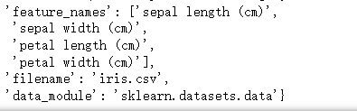
Iris数据集是常用的分类实验数据集，由Fisher, 1936收集整理。Iris也称鸢尾花卉数据集，是一类多重变量分析的数据集。数据集包含150个数据样本，分为3类，每类50个数据，每个数据包含4个属性。可通过花萼长度，花萼宽度，花瓣长度，花瓣宽度4个属性预测鸢尾花卉属于（Setosa，Versicolour，Virginica）三个种类中的哪一类。

该数据集包含了4个属性：
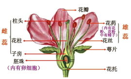
& Sepal.Length（花萼长度），单位是cm;
& Sepal.Width（花萼宽度），单位是cm;
& Petal.Length（花瓣长度），单位是cm;
& Petal.Width（花瓣宽度），单位是cm;
种类：Iris Setosa（山鸢尾）、Iris Versicolour（变色鸢尾），以及Iris Virginica（维吉尼亚鸢尾）。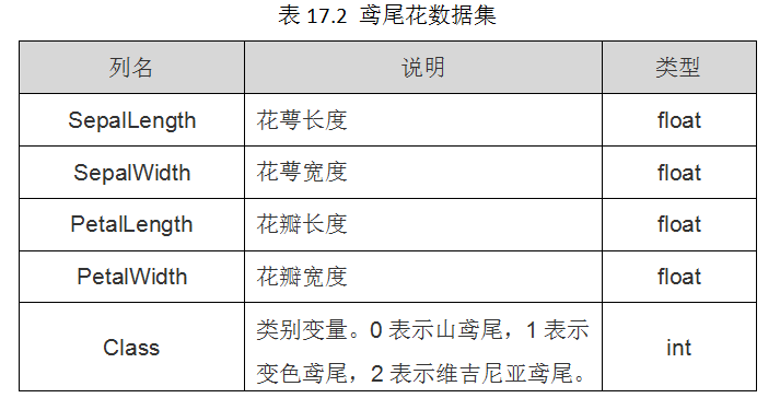

1.2 数据集读取

from sklearn.datasets import load_iris   #导入数据集iris
iris = load_iris()  #载入数据集
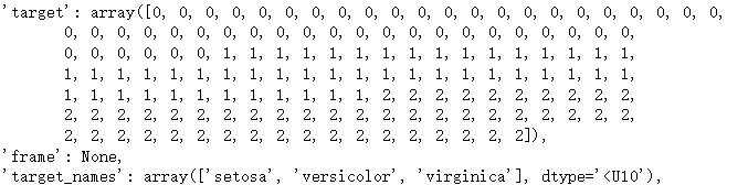
iris

这里的Data是X数据target是Y数据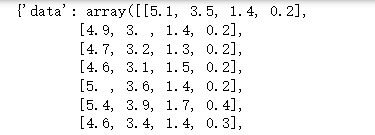

1.3 数据集解析

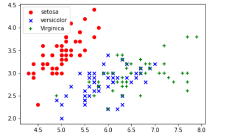
绘制散点图

import matplotlib.pyplot as plt
import numpy as np
DD = iris.data  
X = [x[0] for x in DD]  
Y = [x[1] for x in DD]    
#plt.scatter(X, Y, c=iris.target, marker='x')
plt.scatter(X[:50], Y[:50], color='red', marker='o', label='setosa') #前50个样本
plt.scatter(X[50:100], Y[50:100], color='blue', marker='x', label='versicolor') #中间50个
plt.scatter(X[100:], Y[100:],color='green', marker='+', label='Virginica') #后50个样本
plt.legend(loc=2) #loc=1，2，3，4分别表示label在右上角，左上角，左下角，右下角
plt.show()

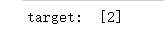
决策树分析（分类）

from sklearn import tree
# 使用决策树训练
X = iris['data']
Y = iris['target']
clf=tree.DecisionTreeClassifier(max_depth=3)
clf.fit(X,Y)
#这里预测当前输入的值的所属分类
print('target: ', [clf.predict([[12,1,-1,10]])[0]])

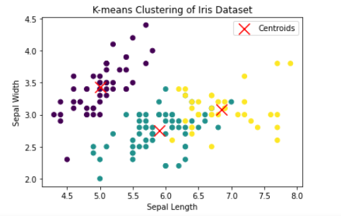
K-means

import numpy as np
import matplotlib.pyplot as plt
from sklearn.cluster import KMeans
from sklearn import datasets
from sklearn.metrics import silhouette_score, adjusted_rand_score

# 设置随机种子
np.random.seed(5)

# 加载鸢尾花数据
iris = datasets.load_iris()
X = iris.data
y_true = iris.target

# 设定聚类簇的个数（鸢尾花数据有3个类别）
k = 3

# 建立KMeans模型
kmeans = KMeans(n_clusters=k, random_state=5)
# 进行聚类
y_pred = kmeans.fit_predict(X)

# 获取簇心
centers = kmeans.cluster_centers_
print("Cluster Centers:\n", centers)

# 计算轮廓系数（越接近1说明聚类越好）
sil_score = silhouette_score(X, y_pred)
print(f'Silhouette Score: {sil_score:.3f}')

# 可视化聚类结果（用前两个特征做二维散点图）
plt.scatter(X[:, 0], X[:, 1], c=y_pred, cmap='viridis', marker='o')
plt.scatter(centers[:, 0], centers[:, 1], c='red', marker='x', s=200, label='Centroids')
plt.xlabel('Sepal Length')
plt.ylabel('Sepal Width')
plt.title('K-means Clustering of Iris Dataset')
plt.legend()
plt.show()

2. 红酒数据集

2.1 数据集介绍

UCI 红酒品质数据集简介

数据集名称：Wine Quality Data Set

来源：由葡萄酒化学分析数据组成，收集自葡萄酒制造商。数据公开在UCI机器学习仓库中。

数据集概述

目的：预测红酒的品质评分（quality），根据其化学属性。

数据特征：包含11个连续型的化学特性和一个品质评分标签。

特征（输入变量）

fixed acidity（固定酸）

volatile acidity（挥发酸）

citric acid（柠檬酸）

residual sugar（残糖）

chlorides（氯化物）

free sulfur dioxide（游离二氧化硫）

total sulfur dioxide（总二氧化硫）

density（密度）

pH（pH值）

sulphates（硫酸盐）

alcohol（酒精浓度）

目标变量（输出）

quality：一个整数评分（通常在0-10之间），由专业品酒师评定。这个评分是对红酒品质的主观评价。

数据特点

样本数：约 1599 个红酒样本。

数据类型：所有特征均为连续值，目标为整数类型的品质评分。

应用：主要用于回归任务（预测酒的品质）或分类（将品质划分为不同类别，比如“低”、“中”、“高”）。

其他信息

用途：适合作为回归与分类的入门项目，用于练习特征工程、模型训练与评估。

挑战：评价的主观性导致数据类别可能存在偏差，且不同评分之间的差异可能不大。

2.2 数据集读取

import pandas as pd

# 数据集文件路径（请根据你的实际路径修改）
file_path = 'winequality-red.csv'

# 读取CSV文件
data = pd.read_csv(file_path, delimiter=';')  # 因为UCI数据集使用';'作为分隔符

# 查看数据的前几行
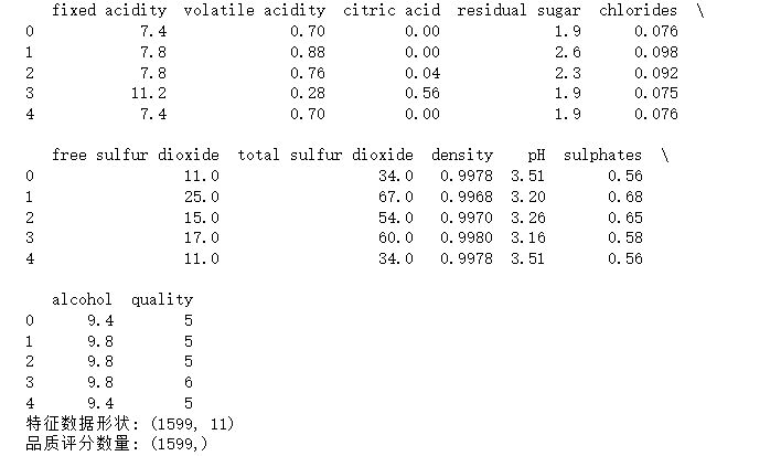
print(data.head())

# 提取特征和标签
X = data.drop('quality', axis=1)     # 特征
y = data['quality']                     # 目标变量（品质）

# 输出数据维度
print(f"特征数据形状: {X.shape}")
print(f"品质评分数量: {y.shape}")

2.3 数据集解析

决策树分类

from sklearn.model_selection import train_test_split
from sklearn.metrics import accuracy_score
from sklearn.tree import DecisionTreeClassifier

# 将品质转换为类别
# 低: 3-4， 中: 5-6， 高: 7及以上
def quality_to_category(q):
    if q <= 4:
        return 'low'
    elif q <= 6:
        return 'medium'
    else:
        return 'high'

y_category = y.apply(quality_to_category)

# 分割数据集
X_train, X_test, y_train, y_test = train_test_split(X, y_category, test_size=0.2, random_state=42)

# 训练决策树分类器
clf = DecisionTreeClassifier(random_state=42)
clf.fit(X_train, y_train)

# 预测
y_pred = clf.predict(X_test)

# 评估
accuracy = accuracy_score(y_test, y_pred)
print(f'分类准确率: {accuracy:.2f}')

分类的使用

import numpy as np

# 已有模型（示例中的clf），假设已训练完毕

def predict_wine_quality(new_sample):
    """
    预测新样本的酒的品质类别（低/中/高）。
    
    参数：
        new_sample: 一个长度等于特征数的数组或列表，如 [fixed acidity, volatile acidity, citric acid, ...]
        
    返回：
        品质类别（字符串）：'low', 'medium', 'high'
    """
    # 转换为2D数组，因为模型需要样本维度为2
    sample = np.array(new_sample).reshape(1, -1)
    # 预测类别
    pred_category = clf.predict(sample)[0]
    return pred_category

# 示例：假设新样本的化学特征如下（请替换为实际数据）
new_sample = [7.4, 0.7, 0.0, 1.9, 0.076, 11, 34, 0.9978, 3.51, 0.56, 9.4]

# 预测
predicted_quality = predict_wine_quality(new_sample)
print(f"预测的酒的品质类别为：{predicted_quality}")

回归测试

from sklearn.linear_model import LinearRegression
from sklearn.metrics import mean_squared_error

# 分割数据
X_train, X_test, y_train, y_test = train_test_split(X, y, test_size=0.2, random_state=42)

# 训练线性回归模型
reg = LinearRegression()
reg.fit(X_train, y_train)

# 预测
y_pred_reg = reg.predict(X_test)

# 评估
mse = mean_squared_error(y_test, y_pred_reg)
print(f'回归均方误差（MSE）: {mse:.2f}')

# 可视化（可选）
import matplotlib.pyplot as plt
plt.scatter(y_test, y_pred_reg, alpha=0.5)
plt.xlabel('真实品质')
plt.ylabel('预测品质')
plt.title('线性回归预测红酒品质')
plt.show()

3. 波士顿房价数据集

3.1 数据集介绍

波士顿房价数据集（Boston Housing Data Set）简介

数据集名称： Boston Housing Data Set

来源： 由哈佛大学的研究人员收集，常用作机器学习中的回归任务示例。

数据集概述

目的： 预测波士顿各个区域的房价中位数（MEDV），帮助分析房价的影响因素。

数据特征： 包含房屋的各种属性和环境指标，反映房价的预测因素。

特征（输入变量）

共13个特征，包括：

CRIM：城镇人均犯罪率

ZN：占地超过25,000平方英尺的住宅用地比例

INDUS：城镇非零售商业用地比例

CHAS：查尔斯河虚拟变量（如果靠近河流，为1，否则为0）

NOX：一氧化氮浓度（区域空气污染指标）

RM：每个住宅的平均房间数

AGE：1940年之前建成的自用房屋比例

DIS：到波士顿五个就业中心的加权距离

RAD：辐射公路的辐射指数（交通便利性指标）

TAX：每一万美元房产税率

PTRATIO：城镇师生比例

B：1000(Bk - 0.63)^2，其中Bk是城镇中黑人比例

LSTAT：人口中地位较低阶层比例

目标变量（输出）

MEDV：房价中位数（以千美元为单位）

数据特点

样本数：大约 506 个样本数据点。

数据类型：大部分特征为连续值。

应用：典型的回归任务，用于预测房价。

其他信息

用途：广泛用于机器学习中的回归模型训练、特征分析和模型评估。

挑战：一些特征存在多重共线性，有利于演示特征选择和模型调优。

3.2 数据集读取

import pandas as pd

# 文件路径，需要你自己指定
file_path = 'boston.csv'

# 读取csv
boston_df = pd.read_csv(file_path)

# 分离特征和目标
X = boston_df.drop('MEDV', axis=1)
y = boston_df['MEDV']

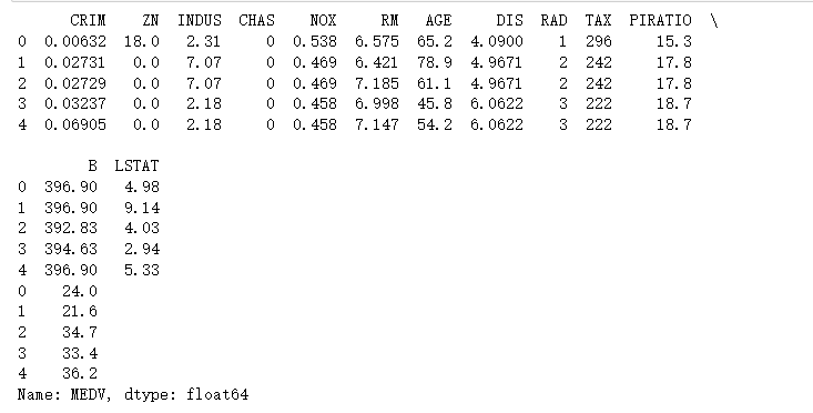
print(X.head())
print(y.head())

3.3 数据集解析

特征选择

from sklearn.feature_selection import RFECV
from sklearn.linear_model import LinearRegression
from sklearn.model_selection import train_test_split

# 拆分训练/测试集
X_train, X_test, y_train, y_test = train_test_split(X, y, test_size=0.2, random_state=42)

# 设定回归模型
lr = LinearRegression()

# 使用RFECV（递归特征消除交叉验证）进行变量选择
selector = RFECV(estimator=lr, step=1, scoring='neg_mean_squared_error', cv=5)

# 执行特征筛选
selector.fit(X_train, y_train)

# 输出选择的特征
selected_features = X.columns[selector.support_]
print("被选择的特征：", list(selected_features))

训练

# 用筛选出的特征训练模型
X_train_sel = selector.transform(X_train)
X_test_sel = selector.transform(X_test)

# 训练线性回归模型
model = LinearRegression()
model.fit(X_train_sel, y_train)

# 预测
y_pred = model.predict(X_test_sel)

评估

from sklearn.metrics import mean_squared_error, r2_score

mse = mean_squared_error(y_test, y_pred)
r2 = r2_score(y_test, y_pred)
print(f"均方误差（MSE）：{mse:.4f}")
print(f"决定系数（R^2）：{r2:.4f}")

对数据进行探索，用seaborn

import pandas as pd
import seaborn as sns
import matplotlib.pyplot as plt

# 读取你本地的csv数据（请确保路径正确）
df = pd.read_csv('boston.csv')  # 替换为你的文件路径

# 假设列名是
# ['CRIM', 'ZN', 'INDUS', 'CHAS', 'NOX', 'RM', 'AGE', 'DIS', 'RAD', 'TAX', 'PTRATIO', 'B', 'LSTAT', 'MEDV']

# 你可以直接用全部特征来绘制pairplot
features = df.columns.drop('MEDV')
data_for_pairplot = df[features].copy()
data_for_pairplot['MEDV'] = df['MEDV']

# 绘制pairplot
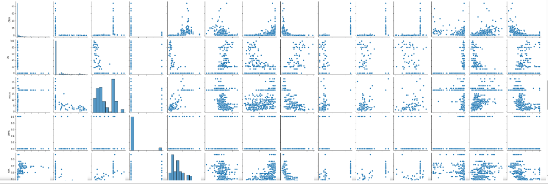
sns.pairplot(data_for_pairplot)
plt.suptitle("使用本地数据集的pairplot", y=1.02)
plt.show()

4. 声纳数据集

4.1 数据集介绍

UCI声纳数据集（Sonar Data Set）简介

数据集名称： Sonar Data Set

来源： UCI机器学习仓库（UC Irvine Machine Learning Repository）

简要概述

目的： 任务是基于声纳信号特征判断目标是“岩石（Rock）”还是“金属（Mine/Metal）”。这是一个二分类问题。

应用背景： 通过分析声波回声信号，判断声源的类型。

数据结构

特征： 每个样本由60个连续的声纳信号特征组成（实际是从声波采样得到的振幅的统计特征）。每个特征都是连续值。

标签： 目标类别为：

“Rock”（岩石），标记为0（或“Mine”）

“Mine”（金属），标记为1

样本数： 总共有208个实例。

主要特点

数据集较小，适合用作二分类任务、模型验证和特征分析。

特征高度相关，适合测试特征选择和降维方法。

信号特征具有一定的复杂性和重复性，实际应用中具有一定的代表性。

典型用途

作为二分类任务的示例数据集

用于机器学习中的特征选择、模型比较

声学信号分析入门

4.2 数据集读取

import pandas as pd

# 读取本地文件（路径自行修改）
df = pd.read_csv('sonar.all-data', header=None)

X = df.iloc[:, :-1]
y = df.iloc[:, -1]

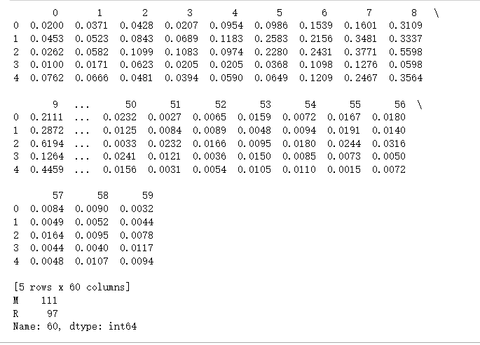
print(X.head())
print(y.value_counts())

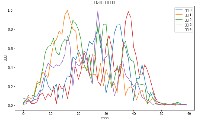
import matplotlib.pyplot as plt

#plt.rcParams['font.family'] = ['Microsoft YaHei']
# 或者设置为黑体
plt.rcParams['font.sans-serif'] = ['SimHei']
# 解决负号显示问题
plt.rcParams['axes.unicode_minus'] = False

# 假设X是你的特征数据，之前已经加载
# 选择前5行数据
rows_to_plot = X.iloc[:5]

# 绘制每一行的折线图
plt.figure(figsize=(10, 6))
for idx, row in rows_to_plot.iterrows():
    plt.plot(row.values, label=f'样本 {idx}')

plt.xlabel('特征索引')
plt.ylabel('特征值')
plt.title('前5行特征的折线图')
plt.legend()
plt.show()

4.3 数据集解析

import pandas as pd
from sklearn.model_selection import train_test_split
from sklearn.ensemble import RandomForestClassifier
from sklearn.metrics import accuracy_score, confusion_matrix, classification_report
from sklearn.preprocessing import LabelEncoder

le = LabelEncoder()
y_encoded = le.fit_transform(y)  # 'Rock' -> 0, 'Mine' -> 1

# 5. 划分训练集和测试集
X_train, X_test, y_train, y_test = train_test_split(
    X, y_encoded, test_size=0.2, random_state=42, stratify=y_encoded
)

# 6. 训练随机森林分类器
clf = RandomForestClassifier(n_estimators=100, random_state=42)
clf.fit(X_train, y_train)

# 7. 预测
y_pred = clf.predict(X_test)

# 8. 评估
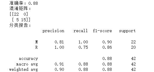
accuracy = accuracy_score(y_test, y_pred)
print(f"准确率：{accuracy:.2f}")

print("混淆矩阵：")
print(confusion_matrix(y_test, y_pred))

print("分类报告：")
print(classification_report(y_test, y_pred, target_names=le.classes_))

5. Mnist手写数字数据集

5.1 数据集介绍

简介

全称：Modified National Institute of Standards and Technology database

用途：广泛用于机器学习、图像识别、深度学习的入门和基准测试

主要内容：手写数字（0-9）图像

数据内容

样本数：总共70,000个样本

训练集：60,000张图像

测试集：10,000张图像

图片尺寸：28×28像素的灰度图

图像格式：

每个数字由像素灰度值组成（0代表白色，255代表黑色）

图像为灰度图，无彩色信息

标签：

每个图像对应一个数字（0到9）

特点

图像简洁，便于快速训练模型

广泛应用于分类任务

已成为ML和DL领域的经典、标准数据集之一

主要用途

图像分类基础入门

测试深度学习模型性能

研究手写识别、图像预处理、特征提取等

5.2 数据集读取

这些数据是在raw文件夹里的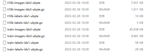

这些文件是 MNIST 数据集 的一部分，通常用于机器学习任务，特别是手写数字的分类。每个文件有特定的作用，具体如下：

t10k-images-idx3-ubyte 和 train-images-idx3-ubyte：

这些文件包含了实际的图像数据，格式是二进制的。每个文件包含了手写数字的图像（就是 MNIST 数据集的图像）。

每张图像的大小是 28x28 像素，灰度图像（即 784 个像素）。

t10k-labels-idx1-ubyte 和 train-labels-idx1-ubyte：

这些文件包含了与图像对应的标签（即每个图像代表的数字）。标签是一个字节的整数，表示图像对应的数字类别（0-9）。

gz 文件：

这些文件是上述文件的压缩版本，使用 .gz 压缩格式。需要先解压缩才能读取内容。

import numpy as np
import struct
import os

data_dir = "raw"

# 读取 images 文件
def read_images(file_name):
    file_path = os.path.join(data_dir, file_name)
    with open(file_path, 'rb') as f:
        magic, num, rows, cols = struct.unpack(">IIII", f.read(16))
        data = np.frombuffer(f.read(), dtype=np.uint8).reshape(num, rows, cols)
    return data

# 读取 labels 文件
def read_labels(file_name):
    file_path = os.path.join(data_dir, file_name)
    with open(file_path, 'rb') as f:
        magic, num = struct.unpack(">II", f.read(8))
        data = np.frombuffer(f.read(), dtype=np.uint8)
    return data

# 读取训练集和测试集
train_images = read_images("train-images-idx3-ubyte")
train_labels = read_labels("train-labels-idx1-ubyte")
test_images  = read_images("t10k-images-idx3-ubyte")
test_labels  = read_labels("t10k-labels-idx1-ubyte")

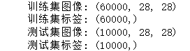
# 输出形状
print("训练集图像:", train_images.shape)
print("训练集标签:", train_labels.shape)
print("测试集图像:", test_images.shape)
print("测试集标签:", test_labels.shape)

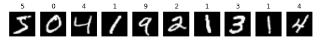
import matplotlib.pyplot as plt

# 显示前 10 张训练集图片
plt.figure(figsize=(10, 2))
for i in range(10):
    plt.subplot(1, 10, i+1)
    plt.imshow(train_images[i], cmap="gray")
    plt.title(str(train_labels[i]))
    plt.axis("off")
plt.show()

5.3 数据集解析

from sklearn.linear_model import LogisticRegression
from sklearn.metrics import accuracy_score
from sklearn.model_selection import train_test_split

# 将 28x28 的图像展开成 1D 向量 (784 维)
X = train_images.reshape(len(train_images), -1)
y = train_labels

# 为了演示快一点，我们只取一部分样本（比如 10000 张）
X_small, _, y_small, _ = train_test_split(X, y, train_size=10000, stratify=y, random_state=42)

# 划分训练集和验证集
X_train, X_val, y_train, y_val = train_test_split(X_small, y_small, test_size=0.2, random_state=42)

# 训练逻辑回归分类器
clf = LogisticRegression(max_iter=1000)
clf.fit(X_train, y_train)

# 预测
y_pred = clf.predict(X_val)

# 准确率
acc = accuracy_score(y_val, y_pred)
print("验证集准确率:", acc)

跑不动，，，为什么？

逻辑回归

from sklearn.linear_model import LogisticRegression
from sklearn.metrics import accuracy_score
from sklearn.model_selection import train_test_split
from sklearn.preprocessing import StandardScaler

# 1. 展平并缩放到 [0,1]
X = train_images.reshape(len(train_images), -1).astype("float32") / 255.0
y = train_labels

# 2. 只取一部分数据（这里取 5000 更快，也足够演示）
X_small, _, y_small, _ = train_test_split(X, y, train_size=5000, stratify=y, random_state=42)

# 3. 再分训练/验证
X_train, X_val, y_train, y_val = train_test_split(X_small, y_small, test_size=0.2, random_state=42)

# 4. 特征标准化（对逻辑回归收敛帮助大）
scaler = StandardScaler()
X_train = scaler.fit_transform(X_train)
X_val = scaler.transform(X_val)

# 5. 训练逻辑回归
clf = LogisticRegression(
    max_iter=300,          # 减少迭代次数
    solver='saga',         # 大数据集/稀疏数据适用
    multi_class='multinomial',
    n_jobs=-1,             # 多核加速
    tol=1e-2               # 提高容忍度，加快收敛
)
clf.fit(X_train, y_train)

# 6. 预测
y_pred = clf.predict(X_val)
acc = accuracy_score(y_val, y_pred)
print("验证集准确率:", acc)

0.877

支持向量机(SVM )

from sklearn.svm import SVC
from sklearn.metrics import accuracy_score
from sklearn.model_selection import train_test_split
from sklearn.preprocessing import StandardScaler

# 1. 展平并缩放到 [0,1]
X = train_images.reshape(len(train_images), -1).astype("float32") / 255.0
y = train_labels

# 2. 只取 3000 条加快演示（你机器快可以调大）
X_small, _, y_small, _ = train_test_split(X, y, train_size=3000, stratify=y, random_state=42)

# 3. 再分训练/验证
X_train, X_val, y_train, y_val = train_test_split(X_small, y_small, test_size=0.2, random_state=42)

# 4. 标准化
scaler = StandardScaler()
X_train = scaler.fit_transform(X_train)
X_val = scaler.transform(X_val)

# 5. 训练 RBF 核 SVM（参数可以调整）
svm_clf = SVC(kernel='rbf', C=5, gamma='scale', cache_size=500)  # cache_size 单位MB
svm_clf.fit(X_train, y_train)

# 6. 预测
y_pred = svm_clf.predict(X_val)

# 7. 输出准确率
acc = accuracy_score(y_val, y_pred)
print("SVM 验证集准确率:", acc)

0.88

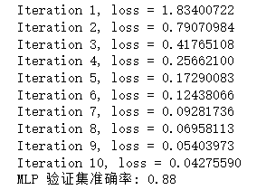
MLP（多层感知机）

from sklearn.neural_network import MLPClassifier
from sklearn.metrics import accuracy_score
from sklearn.model_selection import train_test_split
from sklearn.preprocessing import StandardScaler

# 1. 展平并缩放到 [0,1]
X = train_images.reshape(len(train_images), -1).astype("float32") / 255.0
y = train_labels

# 2. 只取部分数据做演示（比如 2000 张）以提高训练速度
X_small, _, y_small, _ = train_test_split(X, y, train_size=2000, stratify=y, random_state=42)

# 3. 划分训练集和验证集
X_train, X_val, y_train, y_val = train_test_split(X_small, y_small, test_size=0.2, random_state=42)

# 4. 标准化（对 MLP 收敛非常重要）
scaler = StandardScaler()
X_train = scaler.fit_transform(X_train)
X_val = scaler.transform(X_val)

# 5. 建立 MLP 模型，减少迭代次数
mlp_clf = MLPClassifier(
    hidden_layer_sizes=(128, 64),  # 两层隐藏层
    activation='relu',
    solver='adam',
    max_iter=10,        # 迭代次数减少，加速训练
    batch_size=128,     # 调整 batch_size
    learning_rate_init=0.001,
    tol=1e-3,           # 增加容忍度加快收敛
    verbose=True        # 显示训练过程
)

# 6. 训练
mlp_clf.fit(X_train, y_train)

# 7. 预测
y_pred = mlp_clf.predict(X_val)

# 8. 输出准确率
acc = accuracy_score(y_val, y_pred)
print("MLP 验证集准确率:", acc)