本文为李沐老师《动手学深度学习》笔记小结，用于个人复习并记录学习历程，适用于初学者

介绍

在2014年的ImageNet图像识别挑战赛中，一个名叫GoogLeNet的网络架构大放异彩。 GoogLeNet吸收了NiN中串联网络的思想，并在此基础上做了改进。 这篇论文的一个重点是解决了什么样大小的卷积核最合适的问题。 毕竟，以前流行的网络使用小到1×1，大到11×11的卷积核，论文的一个观点是，有时使用不同大小的卷积核组合是有利的。

Inception块

在GoogLeNet中，基本的卷积块被称为Inception块（Inception block）。

框架图

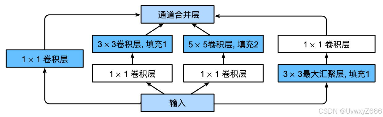
Inception块由四条并行路径组成。 前三条路径使用窗口大小为1×1、3×3和5×5的卷积层，从不同空间大小中提取信息。 中间的两条路径在输入上执行1×1卷积，以减少通道数，从而降低模型的复杂性。 第四条路径使用3×3最大汇聚层，然后使用1×1卷积层来改变通道数。 这四条路径都使用合适的填充来使输入与输出的高和宽一致，最后我们将每条线路的输出在通道维度上连结，并构成Inception块的输出。在Inception块中，通常调整的超参数是每层输出通道数。

代码

import torch
from torch import nn
from torch.nn import functional as F

class Inception(nn.Module):
    # c1--c4是每条路径的输出通道数
    def __init__(self, in_channels, c1, c2, c3, c4, **kwargs):
        super(Inception, self).__init__(**kwargs)
        # 线路1，单1x1卷积层
        self.p1_1 = nn.Conv2d(in_channels, c1, kernel_size=1)
        # 线路2，1x1卷积层后接3x3卷积层
        self.p2_1 = nn.Conv2d(in_channels, c2[0], kernel_size=1)
        self.p2_2 = nn.Conv2d(c2[0], c2[1], kernel_size=3, padding=1)
        # 线路3，1x1卷积层后接5x5卷积层
        self.p3_1 = nn.Conv2d(in_channels, c3[0], kernel_size=1)
        self.p3_2 = nn.Conv2d(c3[0], c3[1], kernel_size=5, padding=2)
        # 线路4，3x3最大汇聚层后接1x1卷积层
        self.p4_1 = nn.MaxPool2d(kernel_size=3, stride=1, padding=1)
        self.p4_2 = nn.Conv2d(in_channels, c4, kernel_size=1)

    def forward(self, x):
        p1 = F.relu(self.p1_1(x))
        p2 = F.relu(self.p2_2(F.relu(self.p2_1(x))))
        p3 = F.relu(self.p3_2(F.relu(self.p3_1(x))))
        p4 = F.relu(self.p4_2(self.p4_1(x)))
        # 在通道维度上连结输出
        return torch.cat((p1, p2, p3, p4), dim=1)

 GoogLeNet模型

框架

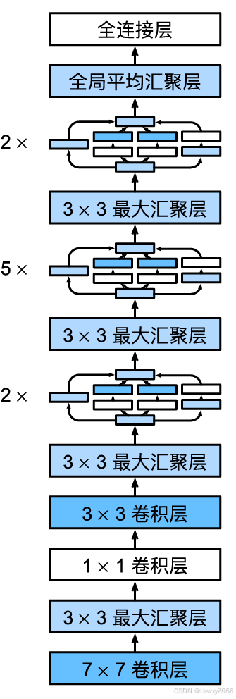
GoogLeNet一共使用9个Inception块和全局平均汇聚层的堆叠来生成其估计值。Inception块之间的最大汇聚层可降低维度。 第一个模块类似于AlexNet和LeNet，Inception块的组合从VGG继承，全局平均汇聚层避免了在最后使用全连接层。

 代码

现在，我们逐一实现GoogLeNet的每个模块。第一个模块使用64个通道、7×7卷积层。

b1 = nn.Sequential(nn.Conv2d(1, 64, kernel_size=7, stride=2, padding=3),
                   nn.ReLU(),
                   nn.MaxPool2d(kernel_size=3, stride=2, padding=1))

 第二个模块使用两个卷积层：第一个卷积层是64个通道、1×1卷积层；第二个卷积层使用将通道数量增加三倍的3×3卷积层。 这对应于Inception块中的第二条路径。

b2 = nn.Sequential(nn.Conv2d(64, 64, kernel_size=1),
                   nn.ReLU(),
                   nn.Conv2d(64, 192, kernel_size=3, padding=1),
                   nn.ReLU(),
                   nn.MaxPool2d(kernel_size=3, stride=2, padding=1))

 第三个模块串联两个完整的Inception块。 第一个Inception块的输出通道数为64+128+32+32=256，四个路径之间的输出通道数量比为64:128:32:32=2:4:1:1。 第二个和第三个路径首先将输入通道的数量分别减少到96/192=1/2和16/192=1/12，然后连接第二个卷积层。第二个Inception块的输出通道数增加到128+192+96+64=480，四个路径之间的输出通道数量比为128:192:96:64=4:6:3:2。 第二条和第三条路径首先将输入通道的数量分别减少到128/256=1/2和32/256=1/8。

b3 = nn.Sequential(Inception(192, 64, (96, 128), (16, 32), 32),
                   Inception(256, 128, (128, 192), (32, 96), 64),
                   nn.MaxPool2d(kernel_size=3, stride=2, padding=1))

第四模块更加复杂， 它串联了5个Inception块，其输出通道数分别是192+208+48+64=512、160+224+64+64=512、128+256+64+64=512、112+288+64+64=528和256+320+128+128=832。 这些路径的通道数分配和第三模块中的类似，首先是含3×3卷积层的第二条路径输出最多通道，其次是仅含1×1卷积层的第一条路径，之后是含5×5卷积层的第三条路径和含3×3最大汇聚层的第四条路径。 其中第二、第三条路径都会先按比例减小通道数。 这些比例在各个Inception块中都略有不同。

b4 = nn.Sequential(Inception(480, 192, (96, 208), (16, 48), 64),
                   Inception(512, 160, (112, 224), (24, 64), 64),
                   Inception(512, 128, (128, 256), (24, 64), 64),
                   Inception(512, 112, (144, 288), (32, 64), 64),
                   Inception(528, 256, (160, 320), (32, 128), 128),
                   nn.MaxPool2d(kernel_size=3, stride=2, padding=1))

 第五模块包含输出通道数为256+320+128+128=832和384+384+128+128=1024的两个Inception块。 其中每条路径通道数的分配思路和第三、第四模块中的一致，只是在具体数值上有所不同。 需要注意的是，第五模块的后面紧跟输出层，该模块同NiN一样使用全局平均汇聚层，将每个通道的高和宽变成1。 最后我们将输出变成二维数组，再接上一个输出个数为标签类别数的全连接层。

b5 = nn.Sequential(Inception(832, 256, (160, 320), (32, 128), 128),
                   Inception(832, 384, (192, 384), (48, 128), 128),
                   nn.AdaptiveAvgPool2d((1,1)),
                   nn.Flatten())

net = nn.Sequential(b1, b2, b3, b4, b5, nn.Linear(1024, 10))

演示各个模块的输出形状：

X = torch.rand(size=(1, 1, 96, 96))
for layer in net:
    X = layer(X)
    print(layer.__class__.__name__,'output shape:\t', X.shape)

 输出：

Sequential output shape:	 torch.Size([1, 64, 24, 24])
Sequential output shape:	 torch.Size([1, 192, 12, 12])
Sequential output shape:	 torch.Size([1, 480, 6, 6])
Sequential output shape:	 torch.Size([1, 832, 3, 3])
Sequential output shape:	 torch.Size([1, 1024])
Linear output shape:	 torch.Size([1, 10])

训练

准备工作

已在之前的文章中多次重复，此处不再赘述。

from IPython import display
import torchvision
from torch.utils import data
from torchvision import transforms
import matplotlib.pyplot as plt

def load_data_fashion_mnist(batch_size, resize=None): 
    """下载Fashion-MNIST数据集，然后将其加载到内存中"""
    trans = [transforms.ToTensor()]
    if resize:
        trans.insert(0, transforms.Resize(resize))
    trans = transforms.Compose(trans)
    mnist_train = torchvision.datasets.FashionMNIST(
        root="../data", train=True, transform=trans, download=0)
    mnist_test = torchvision.datasets.FashionMNIST(
        root="../data", train=False, transform=trans, download=0)
    return (data.DataLoader(mnist_train, batch_size, shuffle=True,
                            num_workers=get_dataloader_workers()),
            data.DataLoader(mnist_test, batch_size, shuffle=False,
                            num_workers=get_dataloader_workers()))
 
def get_dataloader_workers():  
    """使用4个进程来读取数据"""
    return 4

lr, num_epochs, batch_size = 0.1, 10, 128
train_iter, test_iter = load_data_fashion_mnist(batch_size, resize=96)

def accuracy(y_hat, y):  #@save
    """计算预测正确的数量"""
    if len(y_hat.shape) > 1 and y_hat.shape[1] > 1:
        y_hat = y_hat.argmax(axis=1) #找出输入张量（tensor）中最大值的索引
    cmp = y_hat.type(y.dtype) == y
    return float(cmp.type(y.dtype).sum())
class Accumulator:  #@save
    """在n个变量上累加"""
    def __init__(self, n):
        self.data = [0.0] * n
 
    def add(self, *args):
        self.data = [a + float(b) for a, b in zip(self.data, args)]
 
    def reset(self):
        self.data = [0.0] * len(self.data)
 
    def __getitem__(self, idx):
        return self.data[idx]

import matplotlib.pyplot as plt
from matplotlib_inline import backend_inline
 
def use_svg_display(): 
    """使⽤svg格式在Jupyter中显⽰绘图"""
    backend_inline.set_matplotlib_formats('svg')
 
def set_axes(axes, xlabel, ylabel, xlim, ylim, xscale, yscale, legend):
     """设置matplotlib的轴"""
     axes.set_xlabel(xlabel)
     axes.set_ylabel(ylabel)
     axes.set_xscale(xscale)
     axes.set_yscale(yscale)
     axes.set_xlim(xlim)
     axes.set_ylim(ylim)
     if legend:
         axes.legend(legend)
     axes.grid()
 
class Animator:  #@save
    """在动画中绘制数据"""
    def __init__(self, xlabel=None, ylabel=None, legend=None, xlim=None,
                 ylim=None, xscale='linear', yscale='linear',
                 fmts=('-', 'm--', 'g-.', 'r:'), nrows=1, ncols=1,
                 figsize=(3.5, 2.5)):
        # 增量地绘制多条线
        if legend is None:
            legend = []
        use_svg_display()
        self.fig, self.axes = plt.subplots(nrows, ncols, figsize=figsize)
        if nrows * ncols == 1:
            self.axes = [self.axes, ]
        # 使用lambda函数捕获参数
        self.config_axes = lambda: set_axes(
            self.axes[0], xlabel, ylabel, xlim, ylim, xscale, yscale, legend)
        self.X, self.Y, self.fmts = None, None, fmts
 
    def add(self, x, y):
        # 向图表中添加多个数据点
        if not hasattr(y, "__len__"):
            y = [y]
        n = len(y)
        if not hasattr(x, "__len__"):
            x = [x] * n
        if not self.X:
            self.X = [[] for _ in range(n)]
        if not self.Y:
            self.Y = [[] for _ in range(n)]
        for i, (a, b) in enumerate(zip(x, y)):
            if a is not None and b is not None:
                self.X[i].append(a)
                self.Y[i].append(b)
        self.axes[0].cla()
        for x, y, fmt in zip(self.X, self.Y, self.fmts):
            self.axes[0].plot(x, y, fmt)
        self.config_axes()
        display.display(self.fig)
        display.clear_output(wait=True)

def evaluate_accuracy_gpu(net, data_iter, device=None): #@save
    """使用GPU计算模型在数据集上的精度"""
    if isinstance(net, nn.Module):
        net.eval()  # 设置为评估模式
        if not device:
            device = next(iter(net.parameters())).device
    # 正确预测的数量，总预测的数量
    metric = Accumulator(2)
    with torch.no_grad():
        for X, y in data_iter:
            if isinstance(X, list):
                # BERT微调所需的（之后将介绍）
                X = [x.to(device) for x in X]
            else:
                X = X.to(device)
            y = y.to(device)
            metric.add(accuracy(net(X), y), y.numel())
    return metric[0] / metric[1]

import time
class Timer:  #@save
    """记录多次运行时间"""
    def __init__(self):
        self.times = []
        self.start()

    def start(self):
        """启动计时器"""
        self.tik = time.time()

    def stop(self):
        """停止计时器并将时间记录在列表中"""
        self.times.append(time.time() - self.tik)
        return self.times[-1]

    def avg(self):
        """返回平均时间"""
        return sum(self.times) / len(self.times)

    def sum(self):
        """返回时间总和"""
        return sum(self.times)

    def cumsum(self):
        """返回累计时间"""
        return np.array(self.times).cumsum().tolist()

def train_ch6(net, train_iter, test_iter, num_epochs, lr, device):
    """用GPU训练模型(在第六章定义)"""
    def init_weights(m):
        if type(m) == nn.Linear or type(m) == nn.Conv2d:
            nn.init.xavier_uniform_(m.weight)
    net.apply(init_weights)
    print('training on', device)
    net.to(device)
    optimizer = torch.optim.SGD(net.parameters(), lr=lr)
    loss = nn.CrossEntropyLoss()
    animator = Animator(xlabel='epoch', xlim=[1, num_epochs],
                            legend=['train loss', 'train acc', 'test acc'])
    timer, num_batches = Timer(), len(train_iter)
    for epoch in range(num_epochs):
        # 训练损失之和，训练准确率之和，样本数
        metric = Accumulator(3)
        net.train()
        for i, (X, y) in enumerate(train_iter):
            timer.start()
            optimizer.zero_grad()
            X, y = X.to(device), y.to(device)
            y_hat = net(X)
            l = loss(y_hat, y)
            l.backward()
            optimizer.step()
            with torch.no_grad():
                metric.add(l * X.shape[0], accuracy(y_hat, y), X.shape[0])
            timer.stop()
            train_l = metric[0] / metric[2]
            train_acc = metric[1] / metric[2]
            if (i + 1) % (num_batches // 5) == 0 or i == num_batches - 1:
                animator.add(epoch + (i + 1) / num_batches,
                             (train_l, train_acc, None))
        test_acc = evaluate_accuracy_gpu(net, test_iter)
        animator.add(epoch + 1, (None, None, test_acc))
    print(f'loss {train_l:.3f}, train acc {train_acc:.3f}, '
          f'test acc {test_acc:.3f}')
    print(f'{metric[2] * num_epochs / timer.sum():.1f} examples/sec '
          f'on {str(device)}')

def try_gpu(i=0):  #@save
    """如果存在，则返回gpu(i)，否则返回cpu()"""
    if torch.cuda.device_count() >= i + 1:
        return torch.device(f'cuda:{i}')
    return torch.device('cpu')

开始训练

begin = time.time()
train_ch6(net, train_iter, test_iter, num_epochs, lr, try_gpu())
end = time.time()
print(end - begin)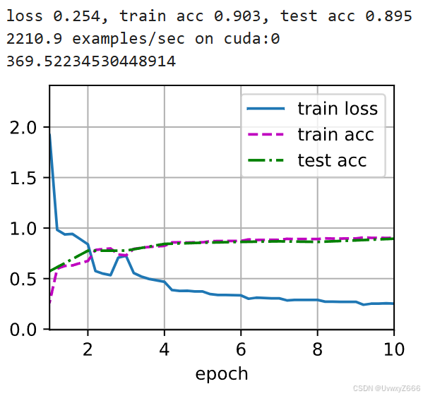

可以看到，GoogLeNet是非常吃计算性能与显存 ，在我这里（4060笔电）运行的时候gpu专用显存吃了1.6G，内存还吃了1G，这还是改小之后的版本。当然，效果也是不错的，在更大的数据集上应该会有更加理想的成果。

小结

• Inception块相当于一个有4条路径的子网络。它通过不同窗口形状的卷积层和最大汇聚层来并行抽取信息，并使用1×1卷积层减少每像素级别上的通道维数从而降低模型复杂度。
• GoogLeNet将多个设计精细的Inception块与其他层（卷积层、全连接层）串联起来。其中Inception块的通道数分配之比是在ImageNet数据集上通过大量的实验得来的。
• GoogLeNet和它的后继者们一度是ImageNet上最有效的模型之一：它以较低的计算复杂度提供了类似的测试精度。