基于强化学习的多码头集卡路径优化
第一个文件的训练过程消耗了最长的训练时间,大约运行了119小时,而剩余文件的训练过程平均只需要40分钟。这种现象发生的原因是,在第一个文件的前750个回合中,DQN从头开始构建学习模型,而接下来的训练过程则利用了之前训练过程中训练好的模型。在ITTRP中,智能体的最终目标是找到一条最优的集卡路径,该路径使集卡的总成本最小(travel cost、空驶成本empty truck trip cost和
Problem Description
问题定义:
- 问题类型: 同车型车辆取送货问题(Homogeneous Vehicle Pickup and Delivery Problem, ITTRP)
- 考虑因素:
- 集卡工作时间的最大可用性
- 延迟订单的罚款
- 节点的时间窗
- 运输订单的截止时间
实验设置:
- 不包括外集卡: 提出的ITTRP版本不考虑外部集卡。
- 实验范围: 釜山新港(Busan New Port,BNP),拥有五个集装箱码头(PNIT、PNC、HJNC、HPNT、BNCT),决策期:24小时,即1440分钟
符号定义:
- 节点集合: L L L
- 集卡集合: T T T
- 客户集合: C C C
- 客户k的订单集合: R k R^k Rk,其中 k k k 是客户的索引。
- 所有订单集合: O = ∪ k ∈ C R k \displaystyle O = \cup_{k \in C} R^k O=∪k∈CRk
- 订单的起始码头: o ( j i k ) ∈ L o(j_i^k) \in L o(jik)∈L
- 订单的目标码头: d ( j i k ) ∈ L d(j_i^k) \in L d(jik)∈L
- 起始码头集合: L s L^s Ls
- 目标码头集合: L d L^d Ld
- 服务时间: 取货点 S j i k , o ( j i k ) S_{j_i^k,o(j_i^k)} Sjik,o(jik) 和送货点 S j i k , d ( j i k ) S_{j_i^k, d(j_i^k)} Sjik,d(jik)的服务时间。
- 订单罚款: p n j i k \displaystyle pn_{j^k_i} pnjik
- 截止日期: d d j i k dd_{j^k_i} ddjik
- 集卡初始位置: i p t ip_t ipt
- 集卡最大工作时间: m x t mx_t mxt
- 集卡使用成本: c s t cs_t cst
- 集卡小时成本: h r t hr_t hrt
目标函数:
- 最小化成本: 使用集卡的成本 min ( ∑ t ∈ T x t c s t + ∑ t ∈ T t m t h r t + ∑ o ∈ O y o p n o ) \displaystyle \min \left( \sum_{t\in T} x_t cs_t + \sum_{t\in T} tm_t hr_t + \sum_{o \in O} y_o pn_o\right) min(t∈T∑xtcst+t∈T∑tmthrt+o∈O∑yopno)
- 成本组成部分:
- 集卡使用成本: ∑ t ∈ T x t c s t \displaystyle \sum_{t \in T} x_t cs_t t∈T∑xtcst
- 集卡工作时间成本: ∑ t ∈ T t m t h r t \displaystyle \sum_{t \in T} tm_t hr_t t∈T∑tmthrt
- 订单延迟罚款: ∑ o ∈ O y o p n o \displaystyle \sum_{o \in O} y_o pn_o o∈O∑yopno
变量定义:
- 集卡是否被雇佣: x t = 1 x_t = 1 xt=1 如果集卡 t t t 被雇佣,否则为 0 0 0。
- 订单是否延迟: y o = 1 y_o = 1 yo=1 如果订单 o o o 在截止日期后执行,否则为 0 0 0。
- 集卡服务时间: t m t tm_t tmt
限制条件:
- Each transport order must be performed.
- Each transport order must be performed by a single truck.
- Each transport order j i k j^k_i jik is ideally performed before its due date, taking into account the service time at the destination locations. The penalty cost p n o , o pn_o, o pno,o ∈ O O O, will be charged if the truck cannot complete a transport order within its due date.
- 每条路线从集卡的起始位置开始。在本例中,所有集卡的初始位置都在一个码头,每辆集卡的下一个起始点是集卡服务的最后一个订单的目的地。从初始位置到订单起始地(对于首次订单分配)所需的时间和成本不包括在目标函数中。
- Pickup and delivery operations are considered as pairing constraints in the transport order
- The pickup vertices are visited before the corresponding delivery vertices (precedence constraints).
- Each location l ∈ L s ∈ L d l ∈ L^s ∈ L^d l∈Ls∈Ld has a given availability time window; hence, the trucks can only arrive at the origin and destination based on their given time windows. When the trucks arrive in advance, they must wait until the location operation time starts and the location is ready for pickup or delivery activities.
A homogeneous vehicle pickup and delivery problem is created using time windows by considering the maximum availability of the truck working hours, penalties for delayed orders, time windows of locations, and due dates of transport orders. The proposed ITTRP version does not consider external trucks, and the site used in our experiment covers only five container terminals. As defined, ITTRP is the process of moving containers between facilities (e.g., container terminals, empty container depots, value-added logistics) within a port. Therefore, we have sets of locations, trucks, and customers represented by L L L, T T T, C C C, respectively, where each customer has a set of requesting orders R k ∈ { j 1 ′ k j 2 ′ k , … , j ∣ R k ∣ k } R^{k} \in\left\{j_{1^{\prime}}^{k} j_{2^{\prime}}^{k}, \ldots, j_{\left|R^{k}\right|}^{k}\right\} Rk∈{j1′kj2′k,…,j∣Rk∣k}. where k k k is the index of the customer. The set of all requesting orders is O = ∪ k ∈ R k O= \displaystyle \cup_{k\in R^k} O=∪k∈Rk. Furthermore, each order, j i k , k ∈ C , i ∈ R k j_i^k,k\in C,i\in R^k jik,k∈C,i∈Rk,has a given origin o ( j i k ) ∈ L o(j_i^k) \in L o(jik)∈L and destination d ( j i k ) ∈ L d(j_i^k) \in L d(jik)∈L. The subsets of the origin and destination are denoted as L s L^s Ls and L d L^d Ld, respectively. Each order must be served by considering the service times at the pickup (i.e., origin) and delivery (i.e., destination) locations, which are denoted as, S j i k , o ( j i k ) S_{j_i^k,o(j_i^k)} Sjik,o(jik) and S j i k , d ( j i k ) S_{j_i^k, d(j_i^k)} Sjik,d(jik), respectively. An associated order penalty p n j i k \displaystyle pn_{j^k_i} pnjik is applied if the transport order cannot be completed before a given due date d d j i k dd_{j^k_i} ddjik. Additionally, each truck t t t ∈ T T T has an initial position, i p t ip_t ipt , a maximum number of working hours, m x t mx_t mxt , a prefixed cost for using a truck, c s t cs_t cst , and variable costs per hour, hr_t . The objective of this problem is to minimize the costs related to the use of trucks, which can be illustrated by the following objective function:
min ( ∑ t ∈ T x t c s t + ∑ t ∈ T t m t h r t + ∑ o ∈ O y o p n o ) \min \left( \sum_{t\in T} x_t cs_t + \sum_{t\in T} tm_t hr_t + \sum_{o \in O} y_o pn_o\right) min(t∈T∑xtcst+t∈T∑tmthrt+o∈O∑yopno)
where x_t is equal to 1 if truck t is hired, 0 otherwise; y_o is equal to 1 if the order o o o is performed after its due date and 0 otherwise. The service time required by a truck t t t for performing all its assigned transport orders is denoted as t m t tm_t tmt . A solution for the ITTRP must satisfy the following feasibility restrictions:
- Each transport order must be performed.
- Each transport order must be performed by a single truck.
- Each transport order j i k j^k_i jik is ideally performed before its due date, taking into account the service time at the destination locations. The penalty cost pn_o, o o o ∈ O O O, will be charged if the truck cannot complete a transport order within its due date.
- Each route begins at the starting position of the truck. In our case, the initial position of all trucks is at a terminal one, and the next starting point of each truck is the destination location of the latest order served by the truck. The time and cost required for moving trucks from the initial location to the order origin (for first-time order assignments) are not considered in the objective function.
- Pickup and delivery operations are considered as pairing constraints in the transport order
- The pickup vertices are visited before the corresponding delivery vertices (precedence constraints).
- Each location l ∈ L s ∈ L d l ∈ L^s ∈ L^d l∈Ls∈Ld has a given availability time window; hence, the trucks can only arrive at the origin and destination based on their given time windows. When the trucks arrive in advance, they must wait until the location operation time starts and the location is ready for pickup or delivery activities.
Proposed method
强化学习是一种通过不断试错和环境反馈来学习决策的机器学习方法。它强调的是如何在给定环境下做出最优决策,而不是简单地从数据中学习模式。通过设计合适的奖励函数,强化学习算法可以训练智能体在复杂的环境中执行特定的任务。强化学习被广泛应用于游戏、机器人控制、自动驾驶、资源管理等领域
RL与其他机器学习技术的区别:
- 监督学习:使用带有标签的训练数据,存在输入和输出之间的映射关系,需要有标记的训练数据来学习模型;训练的目标是使模型能够预测出未见过数据的标签。这通常通过最小化预测标签和真实标签之间的差异来实现,例如使用均方误差(MSE)或交叉熵损失函数;监督学习适用于分类(如垃圾邮件检测)和回归(如房价预测)任务。
- 无监督学习:无监督学习使用没有标签的训练数据,即数据只包含特征,没有对应的标签;训练的目标是发现数据的内在结构或模式。这通常通过聚类(如K-means聚类)或降维(如主成分分析PCA)等技术实现;无监督学习适用于聚类(如市场细分)。
- 强化学习:强化学习通过与环境的交互来学习,而不是从静态的数据集中学习。模型(通常称为智能体)在环境中采取行动,并根据行动的结果(奖励或惩罚)来更新其行为策略;训练的目标是最大化累积奖励,即智能体通过试错学习如何在特定环境中实现最佳行为;强化学习适用于需要决策序列的任务,如游戏、自动驾驶和机器人控制。
智能体与环境的交互:智能体在离散时间步中从可用动作集合中选择动作。选择最佳动作会获得奖励,而选择不佳的动作可能会受到惩罚。奖励是对动作好坏的数值度量,它取决于状态的转移。
强化学习问题通常被定义为马尔可夫决策过程(Markov Decision Process,MDP),是一种用于序列决策制定的经典框架,MDP是一个五元组$< S , A , P , R , γ > $:
- S S S 是状态空间 s ∈ S s \in S s∈S。
- A A A是动作空间 a ∈ A a \in A a∈A。
- P P P是状态转移矩阵。用状态转移矩阵 P P P来描述,在状态 s t s_t st,采取动作 a t a_t at,到达其他状态的概率 p ( s t + 1 ∣ s t = s , a t = a ) p(s_{t+1} \mid s_t=s, a_t=a) p(st+1∣st=s,at=a)。
- R R R是奖励函数, R ( s t = s , a t = a ) = E [ r t ∣ s t = s , a t = a ] R(s_t=s, a_t=a)=\mathbb{E} [r_t \mid s_t = s, a_t=a] R(st=s,at=a)=E[rt∣st=s,at=a]。
- γ \gamma γ是折扣率。
Markov decison process中,Markov代表的是马尔可夫性质(无后效性);decision代表的是策略(Policy),在某个状态s,采取动作a的概率是 π ( a ∣ s ) = P ( a t = a ∣ s t = s ) \pi(a|s)=P(a_t=a \mid s_t = s) π(a∣s)=P(at=a∣st=s);process代表的是状态转移概率
状态设计
在这个问题中,智能体(例如一辆集卡)需要观察当前状态,并在给定时间内选择执行哪个运输订单。状态表示是DRL中的关键组成部分,它通常包括以下信息:
- 当前集卡位置:智能体的初始状态通常包括它在地图上的当前位置。
- 可用运输订单:这包括所有需要运输的订单,每个订单可能具有不同的特征。
- 订单特征:这定义了两个关键因素,包括:
- 当前集卡位置与订单起点之间的距离:这是决定是否选择某个订单的重要因素。
- 当前时间和订单交付时间的gap:智能体需要考虑时间限制来选择最合适的订单。
在设计状态表示时,需要考虑如何有效地编码这些信息,以便智能体可以准确地理解其当前环境并做出决策。例如,可以使用经纬度来表示集卡的当前位置,使用坐标或距离来表示与订单起点的距离,使用时间戳或时间差来表示时间限制。
对订单进行分类:
- OC1:与集卡当前位置(OC1)相似的订单起点的运输订单(transport orders that have an order origin similar to the truck current position)
- OC2:交付时间距当前时间最近的订单(transport orders that have the nearest due date)
- OC3:交付时间距当前时间最远的订单(transport orders that have the farthest due date)
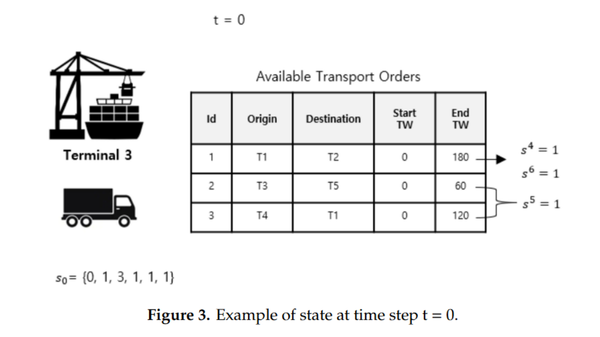
状态空间表示为 S = { s 1 , s 2 , s 3 , s 4 , s 5 , s 6 } t S=\{s^1, s^2, s^3, s^4, s^5, s^6\}_t S={s1,s2,s3,s4,s5,s6}t:
-
s 1 s^1 s1:代表当前时间,以分钟为单位,时间范围为0–1440,为一天。
-
s 2 s^2 s2:代表是否有可选订单,为1则表示至少有一个可选订单。否则为0。
-
s 3 s^3 s3:表示集卡位置,本文研究5个码头的集卡路径优化, s 3 ∈ { 1 , 2 , 3 , 4 , 5 } s^3 \in \{1,2,3,4,5\} s3∈{1,2,3,4,5}
-
s 4 s^4 s4:表示是否有运输订单的起点与集卡当前位置相似,1表示有,0表示没有。(indicates the presence of transport orders that have an order origin similar to the truck’s current position. )
-
s 5 s^5 s5 表明存在具有最近交付时间的订单。The value is zero or one.
-
s 6 s^6 s6 表明存在具有最远交付时间的订单。The value is zero or one.
例如时间步长 t = 0 t=0 t=0时,状态表示为 s 0 = { 0 , 1 , 3 , 1 , 1 , 1 } s_0 = \{0, 1, 3, 1, 1, 1\} s0={0,1,3,1,1,1}
动作设计
动作空间 A = { a 1 , a 2 , a 3 , a 4 , a 5 } t \mathcal{A}=\left\{a^{1}, a^{2}, a^{3}, a^{4}, a^{5}\right\}_{t} A={a1,a2,a3,a4,a5}t
- a 1 a^1 a1:表示空闲(represents idle)
- a 2 a^2 a2:随机选择一个订单
- a 3 a^3 a3:根据OC1选择订单
- a 4 a^4 a4:根据OC2选择订单
- a 5 a^5 a5:根据OC3选择订单
智能体的目标是学习一个策略 π \pi π,以最大化累积奖励。策略π是一个从状态到动作的函数,定义了在状态 s s s中选择动作 a a a的概率: S → p ( A = a ∣ S ) S → p(A = a|S) S→p(A=a∣S)。本文将策略 π π π被表示为一个深度神经网络。根据当前状态值,智能体可以通过策略确定最佳动作值。
奖励函数
在强化学习中,奖励(Reward)是一个核心概念,它代表了智能体(Agent)在特定状态下采取特定动作后从环境中获得的反馈。奖励通常是一个数值,用来量化智能体行为的“好”或“坏”。在ITTRP中,智能体的最终目标是找到一条最优的集卡路径,该路径使集卡的总成本最小(travel cost、空驶成本empty truck trip cost和惩罚成本)。设计每个时间步4种奖励:
-
R ( t ) = 0.01 R(t) = 0.01 R(t)=0.01, 当前时间无可选订单时,选择动作为 a 1 a^1 a1等待,设置较小的奖励为0.01,这是合理的,同时避免智能体认为该动作是最佳动作,防止多次选择。
-
R ( t ) = 0 R(t) = 0 R(t)=0,若选择了不恰当的动作,则奖励设置0,包括:
- T C o i ≥ A T C TC_{o_i}≥ ATC TCoi≥ATC
- 若当前至少有1个订单,选择动作 a 1 a^1 a1
- 若无可选订单,选择动作 a 2 a^2 a2
- 当没有具有OC1特征的订单时,选择动作 a 3 a^3 a3
- 当没有具有OC2特征的订单时,选择动作 a 4 a^4 a4
- 当没有具有OC3特征的订单时,选择动作 a 5 a^5 a5
-
R ( t ) = 1 R(t) = 1 R(t)=1,若智能体选择执行的运输订单的总成本低于之前执行的所有运输订单的总成本的平均值( T C o ≤ A T C TC_o ≤ ATC TCo≤ATC),则设置即使奖励为1。
-
R ( t ) = 25 R(t) = 25 R(t)=25, 如果达到终止状态(所有订单都被服务完成),且 S T C e p s i ≤ A S T C STC_{eps_i} ≤ ASTC STCepsi≤ASTC
- T C o TC_o TCo is the total cost of performing the current transport order, and
- A T C ATC ATC:average of the total cost of performing all previous transport orders, A T C = 1 n ∑ n = 0 i T C o n \displaystyle ATC = \frac{1}{n} \sum_{n=0}^i TC_{o_n} ATC=n1n=0∑iTCon
- S T C e p s i STC_{eps_i} STCepsi:当前回合episode i i i所有已服务运输订单的总成本。(集卡路径优化问题定义为回合任务(episodic task)。强化学习(RL)训练过程执行多个回合(episode)。每个分阶段任务的总成本都必须被计算和评估,以确定智能体是否有所学习上的改进)
- A S T C ASTC ASTC:所有之前回合的 S T C STC STC的均值。
深度Q网络
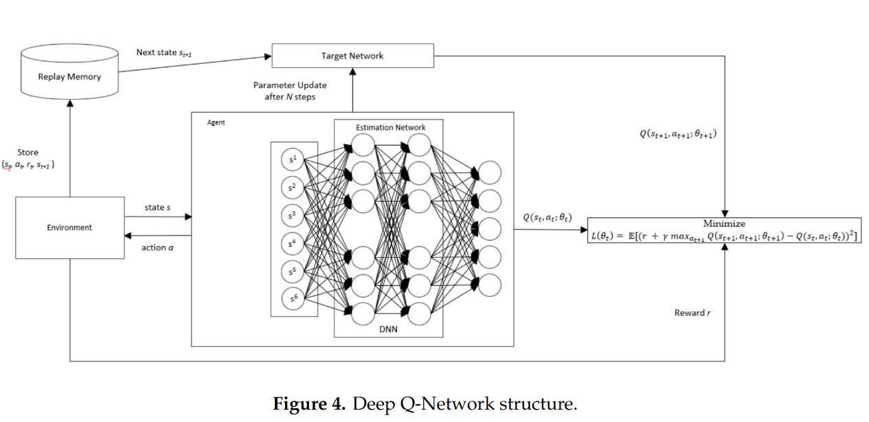
Q学习的表格形式在高维环境中难以收敛,因为它必须无限次地访问所有可能的状态-动作对。深度Q网络(Deep Q-Network,简称DQN)是一种结合了深度学习和Q学习的强化学习算法。它通过使用深度神经网络来近似Q值函数,解决了传统Q学习在处理大规模或连续状态空间时的局限性(high dimensional state and action spaces)。DQN的核心思想是使用深度神经网络来估算Q值函数,并通过优化网络的权重来改进决策策略,这使得DQN能够处理复杂的任务。
具体来说,DQN使用一个深度神经网络来估计Q值函数,这个网络能够接收环境的状态作为输入,并输出在该状态下采取每个可能行动的预期回报。DQN的结构主要包括三个部分:
- Q网络用于训练产生最佳状态-动作价值
- 目标网络则用于计算下一状态下采取的动作所对应的Q值,通过固定目标网络来减少训练过程中的波动
- 经验回放技术(Experience Replay)通过存储智能体的经验并在训练时随机抽取样本,减少了样本间的相关性
**DQN模型结构:**DL in this experiment was developed using KERAS library version 2.3. The DL model has 6 inputs, 2 hidden layers with nine neurons for each layer, and 5 outputs. The input is set to six because, in our case, the input of our DQN should accommodate all elements of the state, which is composed of six elements, while the output of our DQN is the number of possible actions. The number of hidden neurons was determined based on [33], which stated that the number of hidden neurons should comply with the following rule-of-thumb:
- The number of hidden neurons should be between the size of the input layer and the size of the output layer.
- The number of hidden neurons should be 2/3 the size of the input layer, plus the size of the output layer.
- The number of hidden neurons should be less than twice the size of the input layer.
**DQN激活函数。**All hidden layers use a rectified linear activation function, whereas the output layer uses a linear activation function.
DQN超参数设置。The DQN was trained using the configuration with 500 variations of transport data, and each variation running for 1000 episodes:
- Num. of episodes(训练回合数): 750,表示每个回合(或称为“episode”)会运行750个训练步骤。
- Batch-size(批量大小): 32,表示每次从经验回放缓存中随机抽取32个样本进行训练。
- Replay memory(经验回放缓存大小): 100,000,表示用来存储经验元组的缓存可以存储100,000个元组。
- Discount factor(折扣因子) γ: 0.99,用于计算未来奖励的当前价值。
- Learning rate(学习率) α: 0.001,控制梯度下降更新权重的步长。
- Epsilon decay(ε衰减): 0.05,表示ε-greedy策略中ε值在训练过程中逐渐减小的速率。
Experimental Results
在本节中,我们进行了仿真实验以评估所提出方法的性能。该算法使用Python实现,并在配备有Intel® Xeon® CPU E3-1230 v5 3.40 GHz处理器和16 GB内存的PC上运行。我们训练了750个回合的深度Q网络(DQN),并使用了250个文件,每个文件包含285条运输订单数据。训练过程中使用的文件数量代表了运输订单数据的不同变化特征,这些特征可能出现在实际的集装箱码头中。这种数据变化将使我们的DQN智能体学会从不同情况中找到最优策略。整个DQN训练过程大约耗时十一天。第一个文件的训练过程消耗了最长的训练时间,大约运行了119小时,而剩余文件的训练过程平均只需要40分钟。这种现象发生的原因是,在第一个文件的前750个回合中,DQN从头开始构建学习模型,而接下来的训练过程则利用了之前训练过程中训练好的模型。
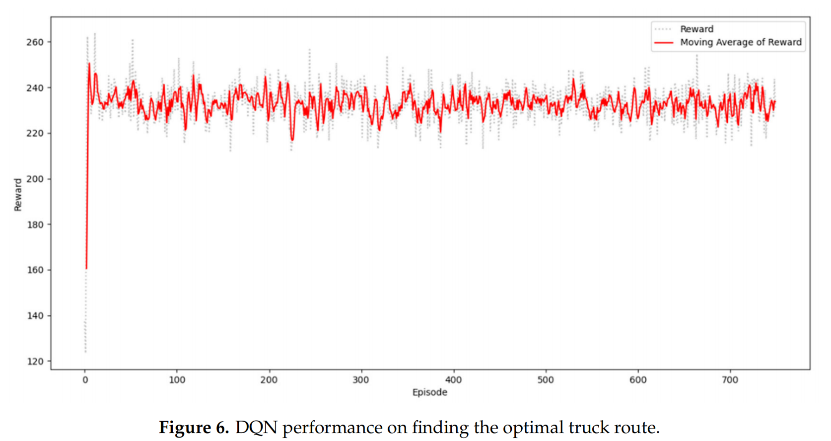
图6展示了深度Q网络(DQN)在寻找最优集卡路线上的表现。x轴代表episode,y轴代表每个episode的累积奖励。从第750个episode开始,奖励显示出显著的增长趋势。DQN仅用100个回合便能够迅速适应环境。
Figure 6 shows the DQN performance on finding the optimal truck route. The x-axis represents the episodes, and the y-axis represents the cumulative rewards per episode. From the 750 episodes, the rewards show a significant increasing trend. The DQN can quickly adapt to the environment within the first 100 episodes.
在这项研究中,最优集卡路线是通过评估所需的总成本来定义的。图7显示了每个episode中总成本的下降趋势。x轴代表episode,y轴代表每个episode中集卡路线的总成本。总成本的变动与奖励趋势一致。当奖励增加时,总成本就会减少。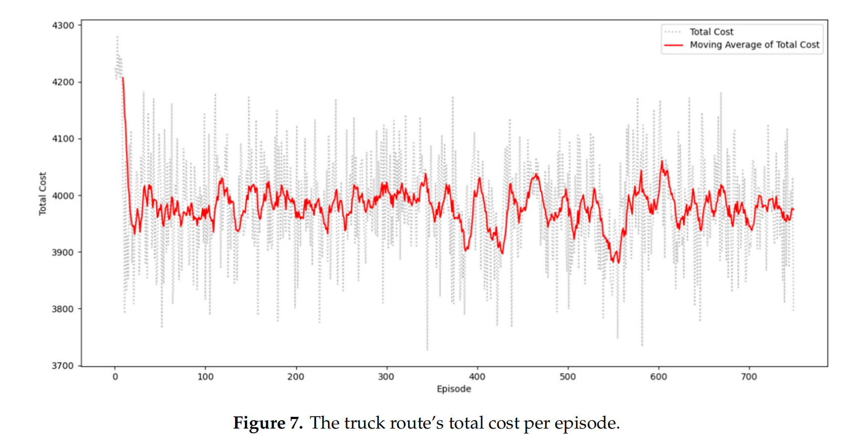
Multi-Agent
the use of single-agent RL led to a sizeable state-action space (33,177,600 combinations of all possible states and actions), thus rendering the agent unable to learn efficiently. Moreover, relying on single-agent RL to achieve two objectives will also decrease the agent’s learning effectiveness. We propose a cooperative multiagent deep RL (CMADRL) that contains two agents focusing on a specific objective to cope with this situation. Figure 4 shows the cooperative multiagent (DRL) architecture used in our case study. Our proposed method’s cooperative term determines that the first and second agents must cooperate to produce a truck route with minimum ETTC and TWC.
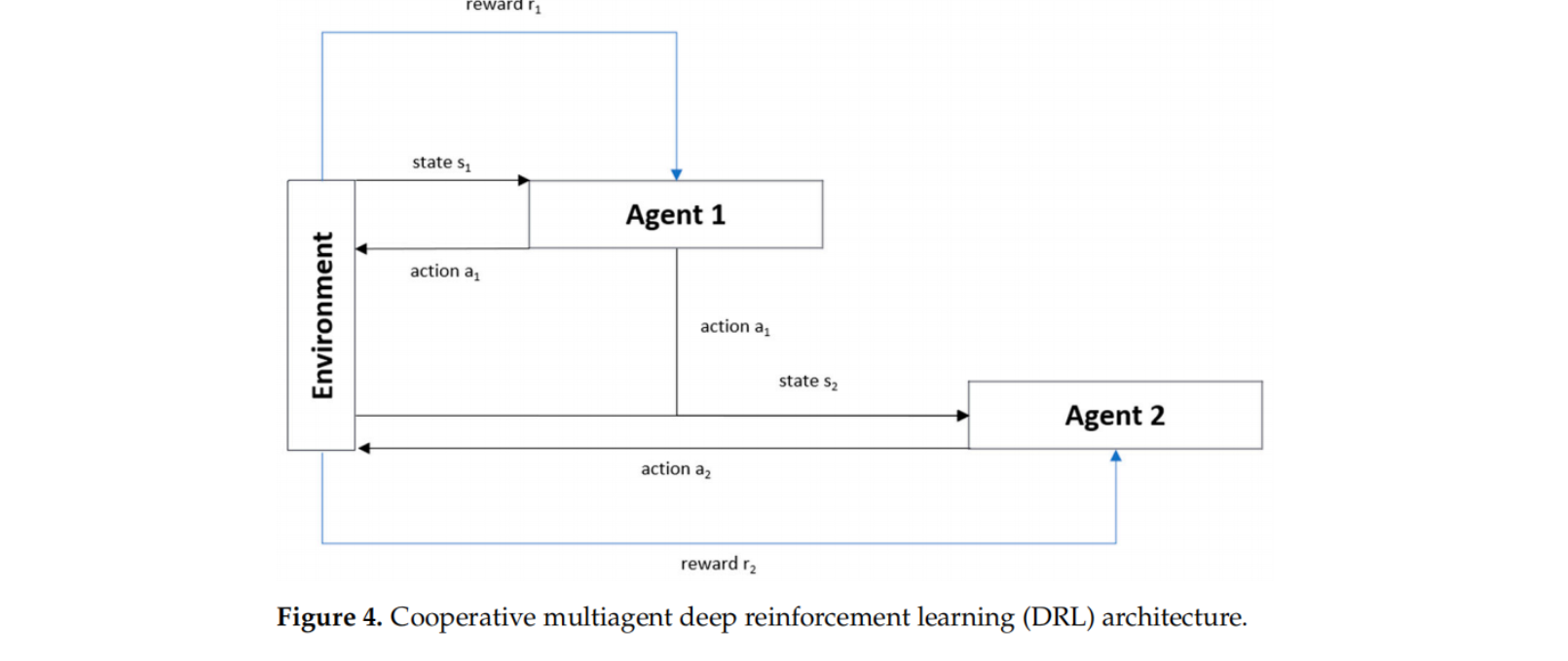
In other words, the decision process is executed in the following sequence: The first agent will evaluate the given state to decide the best action to be taken, and the selected action will then be a part of the second agent’s state. After that, the second agent will decide the best action that should be taken to achieve the second objective. Since the state-action space is considerably large, each agent employs DRL as a policy approximation function.
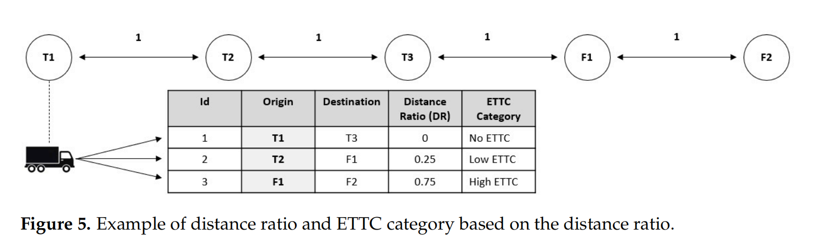
通过Distance Ratio( DR = d i s a n c e ( c p t , o ( j i k ) ) l o n g e s t d i s t a n c e \displaystyle \text{DR}=\frac{disance(cp_t, o(j_i^k))}{longest~distance} DR=longest distancedisance(cpt,o(jik)))表示集卡空驶距离(ETTC)
l o n g e s t d i s t a n c e = max o ( j i k ) ∈ L s d i s a n c e ( c p t , o ( j i k ) ) \displaystyle longest~distance=\max_{o(j_i^k) \in L^s }disance(cp_t, o(j_i^k)) longest distance=o(jik)∈Lsmaxdisance(cpt,o(jik))
Agent1 设计
Agent1 state space S M = { s m 1 , s m 2 , s m 3 , s m 4 , s m 5 } SM=\{sm_1, sm_2, sm_3, sm_4, sm_5\} SM={sm1,sm2,sm3,sm4,sm5},其中
- s m 1 sm_1 sm1 represents the current time in minutes
- s m 2 sm_2 sm2 represents the position of the truck. In our case, we only cover three terminals and two logistics facilities. The value of this element has a range of 1 to 5.
- s m 3 sm_3 sm3 indicates the presence of a TO with DR equal to 0. TOC1
- s m 4 sm_4 sm4 indicates the presence of a TO with DR > 0 and <= 0.50. TOC2
- s m 5 sm_5 sm5 indicates the presence of a TO with DR of more than 0.50. TOC3
Actions A M = { a m 1 , a m 2 , a m 3 } AM=\{am_1, am_2, am_3\} AM={am1,am2,am3}, where:
- am1: choose TO with TOC1 characteristics.
- am2: choose TO with TOC2 characteristics.
- am3: choose TO with TOC3 characteristics
Agent2 设计
在Agent1做出决策后,Agent2根据时间视角来采取行动,选择最小化集卡等待时间的运输订单(TO)。Agent1的决定影响了Agent2可以选择的TO的可用性。假设Agent1选择服务的TO1的起点位置与当前集卡的位置相同(见图5),即T1。因此,Agent2可以选择的可用TO是那些以T1作为原始位置的TO,如图6所示。对于第二个Agent来说,了解TO的等待时间比率(WTR)至关重要,以实现其目标。当集卡提前到达TO的起点时,就会发生集卡等待时间。在这里,Agent2计算两个WTR:原始等待时间比率(OWTR)和目的地等待时间比率(DWTR)。这些比率对于识别TO是否会导致总等待时间(TWC)至关重要:
$$
\begin{array}{c}
\displaystyle O W T R=\frac{o\left(a_{l}\right)-\operatorname{arv}{t}(o)}{W T{\text {threshold }}} \
\displaystyle D W T R=\frac{d\left(a_{l}\right)-\operatorname{arv}{t}(d)}{W T{\text {threshold }}} \
O W T R=\left{\begin{array}{l}
0, \text { where owtr }<0 \
\text { owtr, where owtr }>0
\end{array}\right. \
D W T R=\left{\begin{array}{l}
0, \text { where dwtr }<0 \
\text { dwtr, where dwtr }>0
\end{array}\right.
\end{array}
$$
- o ( a l ) o(a_l) o(al) is the opening time at the TO origin location
- d ( a l ) d(a_l) d(al) is the opening time at the TO destination location
- a r v t ( o ) arv_t(o) arvt(o) is the arrival time of a truck at the TO’s origin
- a r v t ( d ) arv_t(d) arvt(d) is the arrival time of a truck at the TO’s destination
- W T t h r e s h o l d WT_{threshold} WTthreshold is the waiting time threshold indicative of a truck’s maximum acceptable waiting time at the TO origin/destination, 60 min being the default value.
以图三个码头节点(T1、T2、T3)和两个物流设施节点(F1、F2)的5个位置为例,如图6。节点之间的集卡行驶时间为10分钟,集装箱装载需要10分钟。集装当前位置(CTP)位于T1,当前时间为06:00。在那个时间点,有三个可用的运输订单(TOs)选项。所有运输订单的OWTR为0,因为运输订单的起点T1全天候24小时运营。
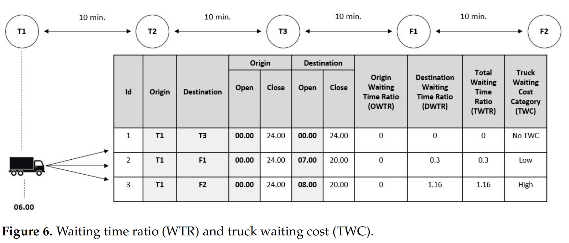
7 × 60 − 6 × 60 + 30 + 10 60 = 0.333333333 \displaystyle \frac{7\times 60 - 6\times 60+30+10}{60}=0.333333333 607×60−6×60+30+10=0.333333333
8 × 60 − 6 × 60 + 40 + 10 60 = 1.16666666666667 \displaystyle \frac{8\times 60 - 6\times 60+40+10}{60}=1.16666666666667 608×60−6×60+40+10=1.16666666666667
在假设每个集装箱装载过程需要10分钟的情况下,我们可以得出运输订单1、2和3的装载等待时间比率(DWTR)分别为0、0.3和1.16。总等待时间比率(TWTR)是OWTR和DWTR的总和。TWTR用于确定等待时间类别(TWC)。如果TWTR等于0,它被归类为无等待时间(NTWC);如果它大于0且小于1,它被归类为低等待时间(LTWC);如果它大于1,它被归类为高等待时间(HTWC)。
State Representation
Agent1 state space S W = { s w 1 , s w 2 , s w 3 , s w 4 , s w 5 } SW=\{sw_1, sw_2, sw_3, sw_4, sw_5\} SW={sw1,sw2,sw3,sw4,sw5},其中
- sw1 means that an action was taken by agent 1.
- sw2 represents the current time in minutes.
- sw3 represents the current position of the truck.
- sw4 indicates the presence of a TO with NTWC characteristics.
- sw5 indicates the presence of a TO with LTWC characteristics.
- sw6 indicates the presence of a TO with HTWC characteristics.
Actions
A W = { a w 1 , a w 2 , a w 3 } AW = \{aw1, aw2, aw3\} AW={aw1,aw2,aw3}, where:
- aw1: choose a TO with NTWC characteristics
- aw2: choose a TO with LTWC characteristics.
- aw3: choose a TO with HTWC characteristics.
Rewards
Agent2的目标是选择最小化总等待时间(TWC)的运输订单;因此,Agent2的奖励设计应该支持Agent的学习并实现目标。Agent2有三种奖励情况,如下所示:
- R(t) = −0.1, if an agent chooses action aw1, aw2, or aw3 when the TO with the corresponding characteristics is not available.
- R(t) = 100, if the selected action results in TWC = 0.
- R(t) = 50, if the selected action results in TWCi <= ATWC, where TWCi is the current TWC(truck waiting cost) and ATWC is the average of all complete TOs’ TWCs.
结论
- 基于RL解决釜山新港5个集装箱码头间集卡调度问题,现实世界的案例应具有与我们的案例研究相似的特征。
- 基于多Agent解决ITTRP多目标问题(空驶集卡行程成本、集卡等待成本)。单一Agent的强化学习(RL)无法高效解决多目标问题,因为这个问题会产生高维的状态-动作空间,需要大量的计算时间。
- 实验结果表明,所提出的CMADRL能够产生比基线算法更好的结果。所提出的方法能够将TWC和ETTC分别比模拟退火(SA)和禁忌搜索(TS)降低高达22.67%和25.45%。
未来挑战
- 提出的方法并非为许多集装箱码头的一般ITTRP设计,因此针对具体问题需要重新设计。
- 作者考虑的ITT问题仅涉及同质性车辆,这无法真实地代表当前通常使用异构车队的现代集装箱码头。
- RL需要大量的训练时间,并且依赖于庞大的训练数据集,现实世界问题中实用性不大。
参考文献
- ADI T N, ISKANDAR Y A, BAE H. Interterminal Truck Routing Optimization Using Deep Reinforcement Learning[J]. Sensors, 2020, 20(20): 5794.
- ADI T N, BAE H, ISKANDAR Y A. Interterminal Truck Routing Optimization Using Cooperative Multiagent Deep Reinforcement Learning[J]. Processes, 2021, 9(10): 1728.

魔乐社区(Modelers.cn) 是一个中立、公益的人工智能社区,提供人工智能工具、模型、数据的托管、展示与应用协同服务,为人工智能开发及爱好者搭建开放的学习交流平台。社区通过理事会方式运作,由全产业链共同建设、共同运营、共同享有,推动国产AI生态繁荣发展。
更多推荐

 9
9 0
0- 0


 已为社区贡献10条内容

所有评论(0)