时间序列预测和时间序列异常检测

import numpy as np
from waveletFunctions import wavelet, wave_signif
import matplotlib.pyplot as plt

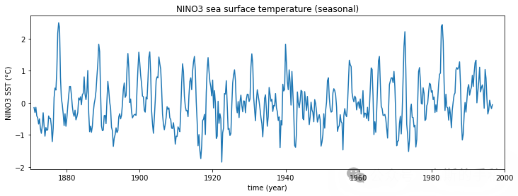
sst = np.loadtxt('sst_nino3.dat')
n = len(sst)
dt = 0.25
time = np.arange(len(sst)) * dt + 1871.0  # time epochs
xlim = ([1870, 2000])


%matplotlib inline
plt.figure(figsize=(12, 4))
plt.plot(time, sst)
plt.xlim(xlim[:])
plt.xlabel('time (year)')
plt.ylabel('NINO3 SST (°C)')
plt.title('NINO3 sea surface temperature (seasonal)')
plt.show()

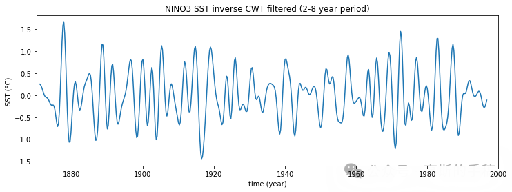
Let us filter this signal such that we keep components with periods between 2-8 years.

Let us use again the function of the inverse wavelet transform which has been written earlier.

def icwt(W, sj, dt, dj=1/8, mother='morlet'):
    """
    Inverse continuous wavelet transform.

    Parameters
    ----------
    W : wavelet transform
    sj : vector of scale indices
    dt : sampling interval
    dj : discrete scale interval, default 0.125.
    mother : mother wavelet (default: Morlet)
    
    Result
    --------
    iW : inverse wavelet transform
    """
    mother = mother.upper()
    if mother == 'MORLET':
        Cd = 0.7785  
        psi0 = 0.751126
    elif mother == 'PAUL': # Paul, m=4
        Cd = 1.132
        psi0 = 1.07894
    elif mother == 'DOG':   # Dog, m=2
        Cd = 3.541
        psi0 = 0.86733
    else:
        raise Error('Mother must be one of Morlet, Paul, DOG')

    a, b = W.shape
    c = sj.size
    if a == c:
        sj = (np.ones([b, 1]) * sj).transpose()
    elif b == c:
        sj = np.ones([a, 1]) * sj
    else:
        raise Warning('Input array dimensions do not match.')

    iW = dj * np.sqrt(dt) / (Cd * psi0) * (
        np.real(W) / np.sqrt(sj)).sum(axis=0)
    return iW

pad = 1  # zero padding (recommended)
dj = 0.125  # 8 sub-octaves (in one octave)
s0 = 2 * dt  # 6 month initial scale
j1 = 7 / dj  # 7 octaves
mother = 'MORLET'

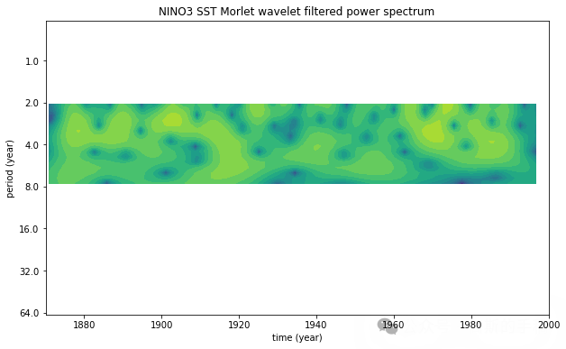
Calculate CWT and determine corrected signal power, filter for 2-8 year periods and make reconstruction of the filtered signal with inverse CWT.

wave, period, scale, coi = wavelet(sst, dt, pad, dj, s0, j1, mother)
scale_ext = np.outer(scale,np.ones(n))
power = (np.abs(wave))**2 /scale_ext  # power spectrum (corrected)

# filtering for periods between 2-8 years
zmask = np.logical_or(scale_ext<2, scale_ext>=8) # zero here
power[zmask] = 0.0
wavethr = np.copy(wave)
wavethr[zmask] = 0.0

# reconstruction by inverse wavelet transform
x = icwt(wavethr, scale, dt, dj, 'morlet')

Plot wavelet map and filtered signal:

import matplotlib

plt.figure(figsize=(10, 6))
levels = np.array([2**i for i in range(-15,5)])
with np.errstate(divide='ignore'):
    CS = plt.contourf(time, period, np.log2(power), len(levels))  
    im = plt.contourf(CS, levels=np.log2(levels))
plt.xlabel('time (year)')
plt.ylabel('period (year)')
plt.title('NINO3 SST Morlet wavelet filtered power spectrum')
plt.xlim(xlim[:])
plt.yscale('log', base=2, subs=None)
plt.ylim([np.min(period), np.max(period)])
ax = plt.gca().yaxis
ax.set_major_formatter(matplotlib.ticker.ScalarFormatter())
plt.ticklabel_format(axis='y', style='plain')
plt.gca().invert_yaxis()
plt.show()

plt.figure(figsize=(12, 4))
plt.plot(time, x)
plt.xlim(xlim[:])
plt.xlabel('time (year)')
plt.ylabel('SST (°C)')
plt.title('NINO3 SST inverse CWT filtered (2-8 year period)')
plt.show()

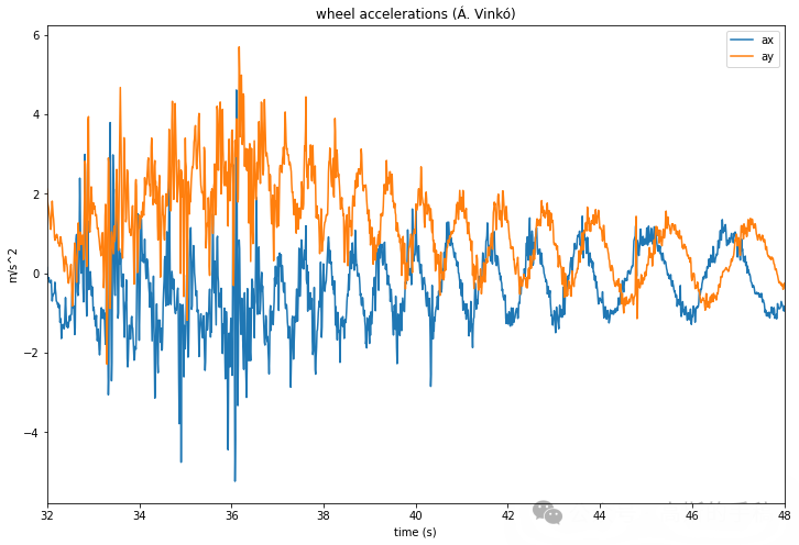
Filtering wheel accelerometry with CWT

aint = np.loadtxt('aint.dat')
tint= aint[:,0]
axi = aint[:,1]
ayi = aint[:,2]
n = len(tint)
dt = 0.01

xlim = [32,48]
plt.figure(figsize=(12, 8))
plt.plot(tint, axi, label='ax')
plt.plot(tint, ayi, label='ay')
plt.xlim(xlim[:])
plt.xlabel('time (s)')
plt.ylabel('m/s^2')
plt.title('wheel accelerations (Á. Vinkó)')
plt.legend()
plt.show()

pad = 1  
dj = 0.125 
s0 = 2*dt
j1 = 10/dj 
mother = 'MORLET'

wave, period, scale, coi = wavelet(axi,dt,pad,dj,s0,j1,mother)
# power spectrum (Compo)
power = (np.abs(wave)) ** 2 
# filtering by thresholding
pvar = np.std(power)**2  # signal variance
lvl = 0.15     # threshold (relative to signal variance)
thr = lvl*pvar
zmask = power <=thr # set zero here
powerthr = np.copy(power)
powerthr[zmask] = 0.0
wavethr = np.copy(wave)
wavethr[zmask] = 0.0

# reconstruction by inverse wavelet transform
axr = icwt(wavethr, scale, dt, dj, 'morlet')

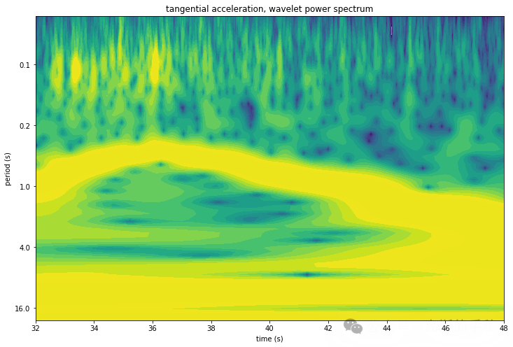
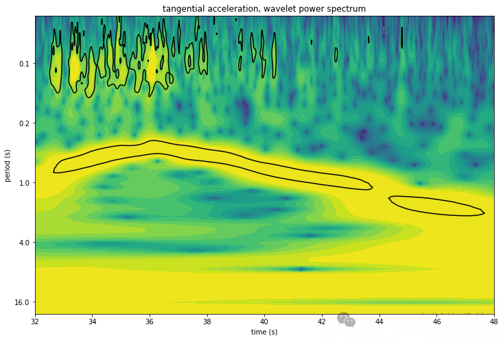
Plot wavelet map of the tangential acceleration component:

plt.figure(figsize=(12, 8))
levels = np.array([2**i for i in range(-15,5)])
CS
 = plt.contourf(tint, period, np.log2(power), len(levels))  im = plt.contourf(CS, levels=np.log2(levels))
plt.xlabel('time (s)')
plt.ylabel('period (s)')
plt.title('tangential acceleration, wavelet power spectrum')
plt.xlim(xlim[:])
plt.yscale('log', base=2, subs=None)
plt.ylim([np.min(period), np.max(period)])
ax = plt.gca().yaxis
ax.set_major_formatter(matplotlib.ticker.ScalarFormatter())
plt.ticklabel_format(axis='y', style='plain')
plt.gca().invert_yaxis()
plt.show()

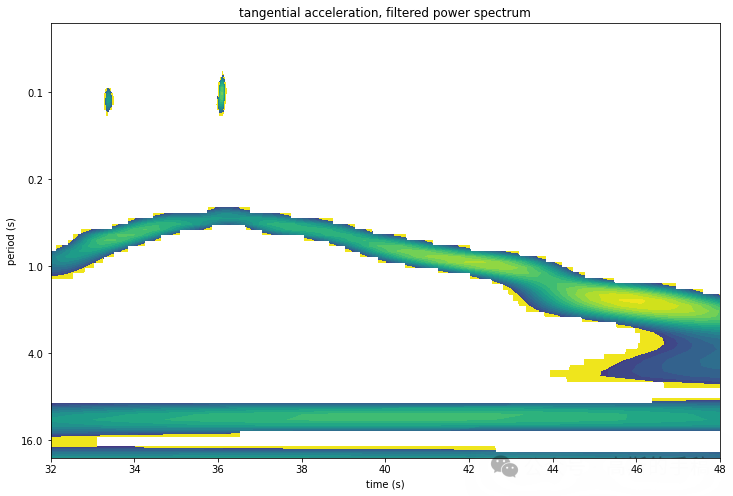
Plot filtered signal and its wavelet map

plt.figure(figsize=(12, 8))
levels = np.array([2**i for i in range(-15,5)])
with np.errstate(divide='ignore'):
    CS
 = plt.contourf(tint, period, np.log2(powerthr), len(levels))      im = plt.contourf(CS, levels=np.log2(levels))
plt.xlabel('time (s)')
plt.ylabel('period (s)')
plt.title('tangential acceleration, filtered power spectrum')
plt.xlim(xlim[:])
plt.yscale('log', base=2, subs=None)
plt.ylim([np.min(period), np.max(period)])
ax = plt.gca().yaxis
ax.set_major_formatter(matplotlib.ticker.ScalarFormatter())
plt.ticklabel_format(axis='y', style='plain')
plt.gca().invert_yaxis()
plt.show()

plt.figure(figsize=(12, 8))
plt.plot(tint, axr)
plt.xlim(xlim[:])
plt.xlabel('time (s)')
plt.ylabel('a_x (m/s^2)')
plt.title('tangential acceleration, inverse WT filtered')
plt.show()

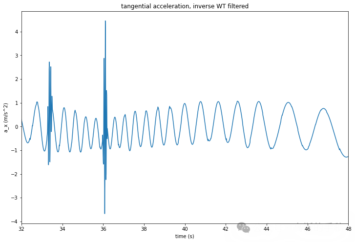
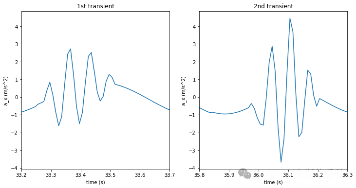
Periodic acceleration transients at 33 s and 36 s are probably due to the slipping driven wheel. This is confirmed by zooming at these places:

plt.figure(figsize=(12, 6))
plt.subplot(121)
plt.plot(tint, axr)
plt.xlim([33.2,33.7])
plt.xlabel('time (s)')
plt.ylabel('a_x (m/s^2)')
plt.title('1st transient')
plt.subplot(122)
plt.plot(tint, axr)
plt.xlim([35.8,36.3])
plt.xlabel('time (s)')
plt.ylabel('a_x (m/s^2)')
plt.title('2nd transient')
plt.show()

plt.figure(figsize=(12, 8))
levels = np.array([2**i for i in range(-15,5)])
CS
 = plt.contourf(tint, period, np.log2(power), len(levels))  im = plt.contourf(CS, levels=np.log2(levels))
plt.xlabel('time (s)')
plt.ylabel('period (s)')
plt.title('tangential acceleration, wavelet power spectrum')
plt.xlim(xlim[:])
plt.yscale('log', base=2, subs=None)
plt.ylim([np.min(period), np.max(period)])
ax = plt.gca().yaxis
ax.set_major_formatter(matplotlib.ticker.ScalarFormatter())
plt.ticklabel_format(axis='y', style='plain')
plt.gca().invert_yaxis()
# 95% significance level
plt.contour(tint, period, sig95, [-99, 1], colors='k')
plt.show()

完整代码可通过学术咨询获得：

魔乐社区

魔乐社区（Modelers.cn) 是一个中立、公益的人工智能社区，提供人工智能工具、模型、数据的托管、展示与应用协同服务，为人工智能开发及爱好者搭建开放的学习交流平台。社区通过理事会方式运作，由全产业链共同建设、共同运营、共同享有，推动国产AI生态繁荣发展。

更多推荐

全家桶集齐！Qwen3.5四款小模型上线魔乐社区，附昇腾全套实践教程

魔乐社区

Pont - 搭建前后端之桥：高效、灵活的接口管理工具

Pont 是一款强大的数据服务层解决方案，它能够帮助开发者快速搭建前后端之间的桥梁，实现接口的高效管理和代码自动生成。无论是新手还是有经验的开发者，都能通过 Pont 轻松处理接口文档、生成类型安全的 API 代码，从而显著提升开发效率。[![Pont 工具标志](https://raw.gitcode.com/gh_mirrors/po/pont/raw/3f1b7d4bbba3fd2dda

魔乐社区

如何快速上手 hvac：HashiCorp Vault Python 客户端零基础入门指南

**hvac** 是 HashiCorp Vault 的 Python 3.X 客户端库，专为开发者提供简单高效的 Vault 交互方式。无论你是需要管理密钥、配置身份验证，还是实现安全的秘密数据存储，hvac 都能帮助你轻松搞定 Vault 的各项操作。本文将带你零基础快速入门，从安装到基础操作，让你在几分钟内即可上手使用这个强大的工具。[![hvac 客户端 Logo](https://r