异常检测---离群点
异常数据离群点检测,算法实战。
首先来简单回顾一下异常检测的基本知识:
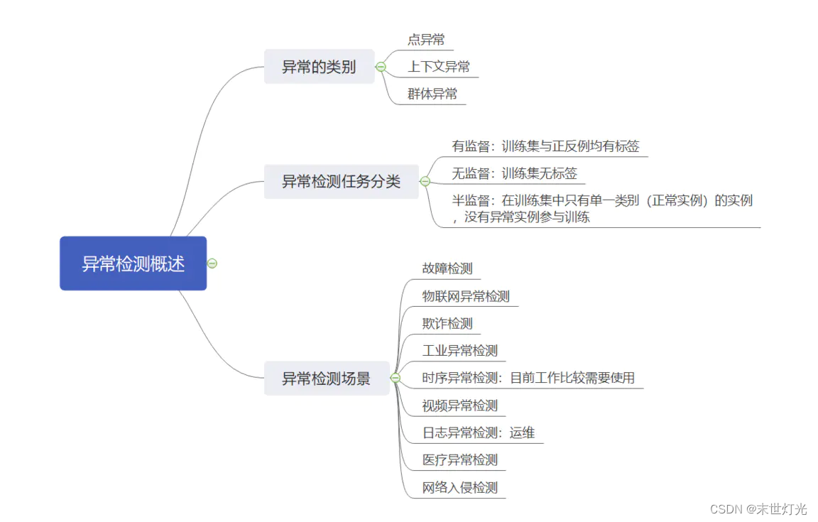


我们使用的是pyod算法工具箱:
1. 包括近40种常见的异常检测算法,比如经典的LOF/LOCI/ABOD以及最新的深度学习如对抗生成模型(GAN)和集成异常检测(outlier ensemble);
2. 支持不同版本的Python:包括2.7和3.5+;支持多种操作系统:windows,macOS和Linux;
3. 简单易用且一致的API,只需要几行代码就可以完成异常检测,方便评估大量算法;
4. 使用JIT和并行化(parallelization)进行优化,加速算法运行及扩展性(scalability),可以处理大量数据;
5. Github地址: GitHub - yzhao062/pyod: A Comprehensive and Scalable Python Library for Outlier Detection (Anomaly Detection)
6. PyPI下载地址: pyod · PyPI
7. 文档与API介绍(英文): pyod 1.0.5 documentation
8. Jupyter Notebook示例(notebooks文件夹): Binder
9. JMLR论文: https://www.jmlr.org/papers/volume20/19-011/19-011.pdf
主要修改地方:
1. 评价函数:
可通过该部分跳转:
def evaluate_print(clf_name, y, y_pred):
    """Utility function for evaluating and printing the results for examples.
    Default metrics include ROC and Precision @ n

    Parameters
    ----------
    clf_name : str
        The name of the detector.

    y : list or numpy array of shape (n_samples,)
        The ground truth. Binary (0: inliers, 1: outliers).

    y_pred : list or numpy array of shape (n_samples,)
        The raw outlier scores as returned by a fitted model.

    """
    from sklearn.metrics import precision_score
    Accuracy = precision_score(y, y_pred, average='micro')
    count1 = 0
    count2 = 0
    for i in range(len(y)):
        if y[i] == 1:
            count1 = count1 + 1
            if y_pred[i] == 1:
                count2 = count2 + 1
    Abnormal_accuracy = count2/count1
    y = column_or_1d(y)
    y_pred = column_or_1d(y_pred)
    check_consistent_length(y, y_pred)
    print('{clf_name} ROC:{roc}, precision @ rank n:{prn}'.format(
        clf_name=clf_name,
        roc=np.round(roc_auc_score(y, y_pred), decimals=4),
        prn=np.round(precision_n_scores(y, y_pred), decimals=4)))
    # AUC的取值范围在0.5和1之间,AUC越接近1.0,检测方法真实性越高;等于0.5时,则真实性最低,无应用价值。
    return np.round(roc_auc_score(y, y_pred), decimals=4), Accuracy, Abnormal_accuracy
2. 建立新文件
# -*- coding: utf-8 -*-
"""Example of using Isolation Forest for outlier detection
"""
from __future__ import division
from __future__ import print_function
import matplotlib.pyplot as plt #导入模块matplotlib.pyplot,并重新命名为plt
import os
import sys
import numpy as np
# temporary solution for relative imports in case pyod is not installed
# if pyod is installed, no need to use the following line
sys.path.append(
os.path.abspath(os.path.join(os.path.dirname("__file__"), '..')))
from pyod.models.iforest import IForest
from pyod.models.abod import ABOD
from pyod.models.alad import ALAD
from pyod.models.auto_encoder import AutoEncoder
from pyod.models.cblof import CBLOF
from pyod.models.cd import CD
from pyod.models.cof import COF
from pyod.models.knn import KNN
from pyod.models.lof import LOF
from pyod.models.pca import PCA
from pyod.models.hbos import HBOS
from pyod.utils.data import generate_data
from pyod.utils.data import evaluate_print
from pyod.utils.example import visualize
def iforest(X_train, X_test, y_train, y_test):
# train IForest detector
clf_name = 'IForest'
clf = IForest()
clf.fit(X_train)
# get the prediction labels and outlier scores of the training data
y_train_pred = clf.labels_ # binary labels (0: inliers, 1: outliers)
y_train_scores = clf.decision_scores_ # raw outlier scores
# get the prediction on the test data
y_test_pred = clf.predict(X_test) # outlier labels (0 or 1)
y_test_scores = clf.decision_function(X_test) # outlier scores
# evaluate and print the results
print("\nOn Test Data:")
roc, Accuracy, Abnormal_accuracy = evaluate_print(clf_name, y_test, y_test_pred)
return y_test_pred, roc, Accuracy, Abnormal_accuracy
def abod(X_train, X_test, y_train, y_test):
# train ABOD detector
clf_name = 'ABOD'
clf = ABOD()
clf.fit(X_train)
# get the prediction labels and outlier scores of the training data
y_train_pred = clf.labels_ # binary labels (0: inliers, 1: outliers)
y_train_scores = clf.decision_scores_ # raw outlier scores
# get the prediction on the test data
y_test_pred = clf.predict(X_test) # outlier labels (0 or 1)
y_test_scores = clf.decision_function(X_test) # outlier scores
# evaluate and print the results
print("\nOn Test Data:")
roc, Accuracy, Abnormal_accuracy = evaluate_print(clf_name, y_test, y_test_pred)
return y_test_pred, roc, Accuracy, Abnormal_accuracy
def alad(X_train, X_test, y_train, y_test):
# train ALAD detector
clf_name = 'ALAD'
clf = ALAD(epochs=100, latent_dim=2,
learning_rate_disc=0.0001,
learning_rate_gen=0.0001,
dropout_rate=0.2,
add_recon_loss=False,
lambda_recon_loss=0.05,
add_disc_zz_loss=True,
dec_layers=[75, 100],
enc_layers=[100, 75],
disc_xx_layers=[100, 75],
disc_zz_layers=[25, 25],
disc_xz_layers=[100, 75],
spectral_normalization=False,
activation_hidden_disc='tanh', activation_hidden_gen='tanh',
preprocessing=True, batch_size=200, contamination=contamination)
clf.fit(X_train)
# get the prediction labels and outlier scores of the training data
y_train_pred = clf.labels_ # binary labels (0: inliers, 1: outliers)
y_train_scores = clf.decision_scores_ # raw outlier scores
# get the prediction on the test data
y_test_pred = clf.predict(X_test) # outlier labels (0 or 1)
y_test_scores = clf.decision_function(X_test) # outlier scores
# evaluate and print the results
print("\nOn Test Data:")
roc, Accuracy, Abnormal_accuracy = evaluate_print(clf_name, y_test, y_test_pred)
return y_test_pred, roc, Accuracy, Abnormal_accuracy
def auto_encoder(X_train, X_test, y_train, y_test):
# train AutoEncoder detector
clf_name = 'AutoEncoder'
clf = AutoEncoder(epochs=30, contamination=contamination)
clf.fit(X_train)
# get the prediction labels and outlier scores of the training data
y_train_pred = clf.labels_ # binary labels (0: inliers, 1: outliers)
y_train_scores = clf.decision_scores_ # raw outlier scores
# get the prediction on the test data
y_test_pred = clf.predict(X_test) # outlier labels (0 or 1)
y_test_scores = clf.decision_function(X_test) # outlier scores
# evaluate and print the results
print("\nOn Test Data:")
roc, Accuracy, Abnormal_accuracy = evaluate_print(clf_name, y_test, y_test_pred)
return y_test_pred, roc, Accuracy, Abnormal_accuracy
def cblof(X_train, X_test, y_train, y_test):
# train CBLOF detector
clf_name = 'CBLOF'
clf = CBLOF(random_state=42)
clf.fit(X_train)
# get the prediction labels and outlier scores of the training data
y_train_pred = clf.labels_ # binary labels (0: inliers, 1: outliers)
y_train_scores = clf.decision_scores_ # raw outlier scores
# get the prediction on the test data
y_test_pred = clf.predict(X_test) # outlier labels (0 or 1)
y_test_scores = clf.decision_function(X_test) # outlier scores
# evaluate and print the results
print("\nOn Test Data:")
roc, Accuracy, Abnormal_accuracy = evaluate_print(clf_name, y_test, y_test_pred)
return y_test_pred, roc, Accuracy, Abnormal_accuracy
def cd(X_train, X_test, y_train, y_test):
# train HBOS detector
clf_name = 'CD'
clf = CD()
clf.fit(X_train, y_train)
# get the prediction labels and outlier scores of the training data
y_train_pred = clf.labels_ # binary labels (0: inliers, 1: outliers)
y_train_scores = clf.decision_scores_ # raw outlier scores
# get the prediction on the test data
y_test_pred = clf.predict(np.append(X_test, y_test.reshape(-1, 1), axis=1)) # outlier labels (0 or 1)
y_test_scores = clf.decision_function(np.append(X_test, y_test.reshape(-1, 1), axis=1)) # outlier scores
# evaluate and print the results
print("\nOn Test Data:")
roc, Accuracy, Abnormal_accuracy = evaluate_print(clf_name, y_test, y_test_pred)
return y_test_pred, roc, Accuracy, Abnormal_accuracy
def cof(X_train, X_test, y_train, y_test):
# train COF detector
clf_name = 'COF'
clf = COF(n_neighbors=30)
clf.fit(X_train)
# get the prediction labels and outlier scores of the training data
y_train_pred = clf.labels_ # binary labels (0: inliers, 1: outliers)
y_train_scores = clf.decision_scores_ # raw outlier scores
# get the prediction on the test data
y_test_pred = clf.predict(X_test) # outlier labels (0 or 1)
y_test_scores = clf.decision_function(X_test) # outlier scores
# evaluate and print the results
print("\nOn Test Data:")
roc, Accuracy, Abnormal_accuracy = evaluate_print(clf_name, y_test, y_test_pred)
return y_test_pred, roc, Accuracy, Abnormal_accuracy
def lof(X_train, X_test, y_train, y_test):
# train LOF detector
clf_name = 'LOF'
clf = LOF()
clf.fit(X_train)
# get the prediction labels and outlier scores of the training data
y_train_pred = clf.labels_ # binary labels (0: inliers, 1: outliers)
y_train_scores = clf.decision_scores_ # raw outlier scores
# get the prediction on the test data
y_test_pred = clf.predict(X_test) # outlier labels (0 or 1)
y_test_scores = clf.decision_function(X_test) # outlier scores
# evaluate and print the results
print("\nOn Test Data:")
roc, Accuracy, Abnormal_accuracy = evaluate_print(clf_name, y_test, y_test_pred)
return y_test_pred, roc, Accuracy, Abnormal_accuracy
def knn(X_train, X_test, y_train, y_test):
# train kNN detector
clf_name = 'KNN'
clf = KNN()
clf.fit(X_train)
# get the prediction labels and outlier scores of the training data
y_train_pred = clf.labels_ # binary labels (0: inliers, 1: outliers)
y_train_scores = clf.decision_scores_ # raw outlier scores
# get the prediction on the test data
y_test_pred = clf.predict(X_test) # outlier labels (0 or 1)
y_test_scores = clf.decision_function(X_test) # outlier scores
# evaluate and print the results
print("\nOn Test Data:")
roc, Accuracy, Abnormal_accuracy = evaluate_print(clf_name, y_test, y_test_pred)
return y_test_pred, roc, Accuracy, Abnormal_accuracy
def pca(X_train, X_test, y_train, y_test):
# train PCA detector
clf_name = 'PCA'
clf = PCA(n_components=3)
clf.fit(X_train)
# get the prediction labels and outlier scores of the training data
y_train_pred = clf.labels_ # binary labels (0: inliers, 1: outliers)
y_train_scores = clf.decision_scores_ # raw outlier scores
# get the prediction on the test data
y_test_pred = clf.predict(X_test) # outlier labels (0 or 1)
y_test_scores = clf.decision_function(X_test) # outlier scores
# evaluate and print the results
print("\nOn Test Data:")
roc, Accuracy, Abnormal_accuracy = evaluate_print(clf_name, y_test, y_test_pred)
return y_test_pred, roc, Accuracy, Abnormal_accuracy
def hbos(X_train, X_test, y_train, y_test):
# train HBOS detector
clf_name = 'HBOS'
clf = HBOS()
clf.fit(X_train)
# get the prediction labels and outlier scores of the training data
y_train_pred = clf.labels_ # binary labels (0: inliers, 1: outliers)
y_train_scores = clf.decision_scores_ # raw outlier scores
# get the prediction on the test data
y_test_pred = clf.predict(X_test) # outlier labels (0 or 1)
y_test_scores = clf.decision_function(X_test) # outlier scores
# evaluate and print the results
print("\nOn Test Data:")
roc, Accuracy, Abnormal_accuracy = evaluate_print(clf_name, y_test, y_test_pred)
return y_test_pred, roc, Accuracy, Abnormal_accuracy
if __name__ == "__main__":
contamination = 0.3 # percentage of outliers
n_train = 2000 # number of training points
n_test = 200 # number of testing points
a = []
for i in range(n_test):
a.append(i)
# Generate sample data
X_train, X_test, y_train, y_test = \
generate_data(n_train=n_train,
n_test=n_test,
n_features=200,
contamination=contamination,
random_state=42)
number = X_test.T[0]
plt.rcParams['font.sans-serif'] = ['SimHei'] # 用来正常显示中文标签
plt.rcParams['axes.unicode_minus'] = False # 用来正常显示负号
plt.figure(figsize=(8, 8), dpi=80)
plt.figure(1)
# 真实数据显示
ax1 = plt.subplot(2,2,1)
ax1.plot(X_test, linewidth=2)
ax1.set_title("actual")
ax1.fill_between(a, np.min(X_test), np.max(X_test),where=y_test==1.0, color='r', alpha=.4)
# 随机森林
y_test_pred, roc, Accuracy, Abnormal_accuracy = iforest(X_train, X_test, y_train, y_test)
ax2 = plt.subplot(2,2,2)
ax2.plot(X_test, linewidth=2)
ax2.set_title("iforest")
ax2.set_xlabel("roc:" + str(roc) + " " + "Accuracy:" + str(Accuracy) + " " + "Abnormal_accuracy:" + str(Abnormal_accuracy))
ax2.fill_between(a, np.min(X_test), np.max(X_test), where=y_test_pred == 1.0, color='r', alpha=.4)
# 基于角度的离群值检测
y_test_pred, roc, Accuracy, Abnormal_accuracy = abod(X_train, X_test, y_train, y_test)
ax3 = plt.subplot(2,2,3)
ax3.plot(X_test, linewidth=2)
ax3.set_title("abod")
ax3.set_xlabel("roc:" + str(roc) + " " + "Accuracy:" + str(Accuracy) + " " + "Abnormal_accuracy:" + str(Abnormal_accuracy))
ax3.fill_between(a, np.min(X_test), np.max(X_test), where=y_test_pred == 1.0, color='r', alpha=.4)
# 基于双指向性GAN异常检测的方法ALAD,使用对抗学习到的特征的重建误差决定样本是否异常。
y_test_pred, roc, Accuracy, Abnormal_accuracy = alad(X_train, X_test, y_train, y_test)
ax4 = plt.subplot(2,2,4)
ax4.plot(X_test, linewidth=2)
ax4.set_title("alad")
ax4.set_xlabel("roc:" + str(roc) + " " + "Accuracy:" + str(Accuracy) + " " + "Abnormal_accuracy:" + str(Abnormal_accuracy))
ax4.fill_between(a, np.min(X_test), np.max(X_test), where=y_test_pred == 1.0, color='r', alpha=.4)
# 第二个图
plt.figure(2)
# 自动编码器
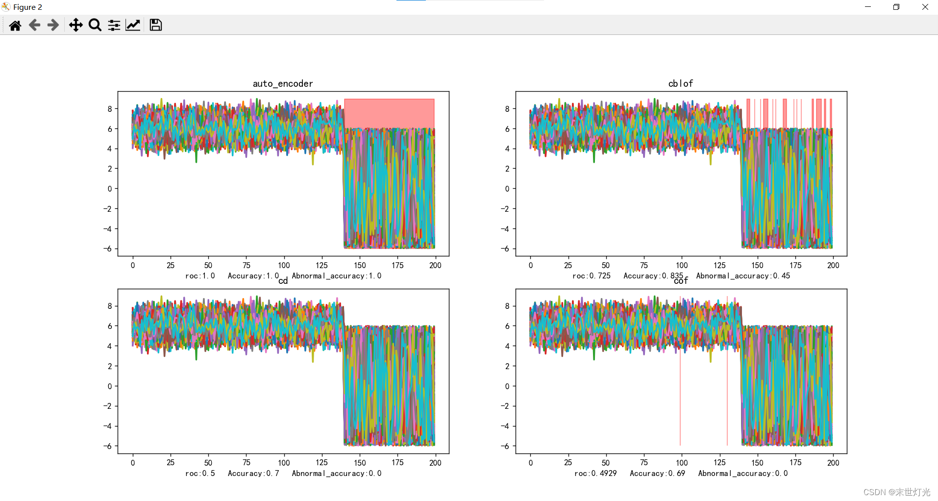
y_test_pred, roc, Accuracy, Abnormal_accuracy = auto_encoder(X_train, X_test, y_train, y_test)
ax5 = plt.subplot(2, 2, 1)
ax5.plot(X_test, linewidth=2)
ax5.set_title("auto_encoder")
ax5.set_xlabel("roc:" + str(roc) + " " + "Accuracy:" + str(Accuracy) + " " + "Abnormal_accuracy:" + str(Abnormal_accuracy))
ax5.fill_between(a, np.min(X_test), np.max(X_test), where=y_test_pred == 1.0, color='r', alpha=.4)
'''CBLOF也是一种基于其他机器学习算法的异常检测算法。说到基于,就是CBLOF名字里面的B~Based。而他基于的是其他的聚类算法,
所以他就是Cluster-Based。LOF三个字母是Local Outlier Factor,本地异常因子。
合起来CBLOF 就是 Cluster-based Local Outlier Factor,基于聚类的本地异常因子。
'''
y_test_pred, roc, Accuracy, Abnormal_accuracy = cblof(X_train, X_test, y_train, y_test)
ax6 = plt.subplot(2, 2, 2)
ax6.plot(X_test, linewidth=2)
ax6.set_title("cblof")
ax6.set_xlabel("roc:" + str(roc) + " " + "Accuracy:" + str(Accuracy) + " " + "Abnormal_accuracy:" + str(Abnormal_accuracy))
ax6.fill_between(a, np.min(X_test), np.max(X_test), where=y_test_pred == 1.0, color='r', alpha=.4)
# cd cooks distance
y_test_pred, roc, Accuracy, Abnormal_accuracy = cd(X_train, X_test, y_train, y_test)
ax7 = plt.subplot(2, 2, 3)
ax7.plot(X_test, linewidth=2)
ax7.set_title("cd")
ax7.set_xlabel(
"roc:" + str(roc) + " " + "Accuracy:" + str(Accuracy) + " " + "Abnormal_accuracy:" + str(Abnormal_accuracy))
ax7.fill_between(a, np.min(X_test), np.max(X_test), where=y_test_pred == 1.0, color='r', alpha=.4)
# LOF中计算距离是用的欧式距离,也是默认了数据是球状分布,而COF的局部密度是根据最短路径方法求出的,也叫做链式距离。
y_test_pred, roc, Accuracy, Abnormal_accuracy = cof(X_train, X_test, y_train, y_test)
ax8 = plt.subplot(2, 2, 4)
ax8.plot(X_test, linewidth=2)
ax8.set_title("cof")
ax8.set_xlabel(
"roc:" + str(roc) + " " + "Accuracy:" + str(Accuracy) + " " + "Abnormal_accuracy:" + str(Abnormal_accuracy))
ax8.fill_between(a, np.min(X_test), np.max(X_test), where=y_test_pred == 1.0, color='r', alpha=.4)
# 第三个图
plt.figure(3)
# knn
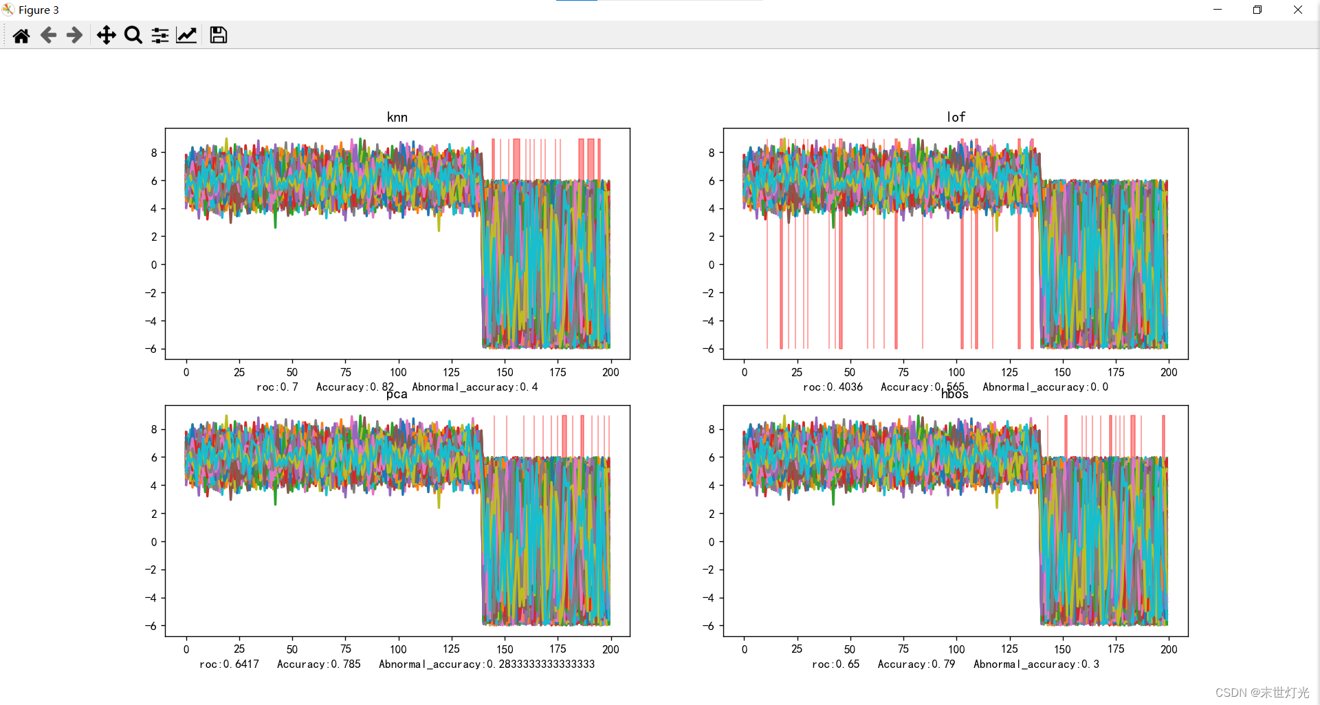
y_test_pred, roc, Accuracy, Abnormal_accuracy = knn(X_train, X_test, y_train, y_test)
ax9 = plt.subplot(2, 2, 1)
ax9.plot(X_test, linewidth=2)
ax9.set_title("knn")
ax9.set_xlabel(
"roc:" + str(roc) + " " + "Accuracy:" + str(Accuracy) + " " + "Abnormal_accuracy:" + str(Abnormal_accuracy))
ax9.fill_between(a, np.min(X_test), np.max(X_test), where=y_test_pred == 1.0, color='r', alpha=.4)
# lof
y_test_pred, roc, Accuracy, Abnormal_accuracy = lof(X_train, X_test, y_train, y_test)
ax10 = plt.subplot(2, 2, 2)
ax10.plot(X_test, linewidth=2)
ax10.set_title("lof")
ax10.set_xlabel(
"roc:" + str(roc) + " " + "Accuracy:" + str(Accuracy) + " " + "Abnormal_accuracy:" + str(Abnormal_accuracy))
ax10.fill_between(a, np.min(X_test), np.max(X_test), where=y_test_pred == 1.0, color='r', alpha=.4)
# 基于矩阵分解的异常点检测方法的主要思想是利用主成分分析(PCA)去寻找那些违反了数据之间相关性的异常点。
y_test_pred, roc, Accuracy, Abnormal_accuracy = pca(X_train, X_test, y_train, y_test)
ax11 = plt.subplot(2, 2, 3)
ax11.plot(X_test, linewidth=2)
ax11.set_title("pca")
ax11.set_xlabel(
"roc:" + str(roc) + " " + "Accuracy:" + str(Accuracy) + " " + "Abnormal_accuracy:" + str(Abnormal_accuracy))
ax11.fill_between(a, np.min(X_test), np.max(X_test), where=y_test_pred == 1.0, color='r', alpha=.4)
'''HBOS全名为:Histogram-based Outlier Score。它是一种单变量方法的组合,不能对特征之间的依赖关系进行建模,
但是计算速度较快,对大数据集友好,其基本假设是数据集的每个维度相互独立,然后对 每个维度进行区间(bin)划分,
区间的密度越高,异常评分越低。'''
y_test_pred, roc, Accuracy, Abnormal_accuracy = hbos(X_train, X_test, y_train, y_test)
ax12 = plt.subplot(2, 2, 4)
ax12.plot(X_test, linewidth=2)
ax12.set_title("hbos")
ax12.set_xlabel(
"roc:" + str(roc) + " " + "Accuracy:" + str(Accuracy) + " " + "Abnormal_accuracy:" + str(Abnormal_accuracy))
ax12.fill_between(a, np.min(X_test), np.max(X_test), where=y_test_pred == 1.0, color='r', alpha=.4)
plt.show()
试验介绍
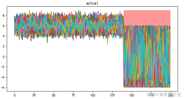
数据样例:
使用数据生成器,生成200个特征的数据,训练数据2000条,测试数据200条,异常数据比例设置为0.3,即前70%为正常数据,后30%为异常数据。
注:生成合成数据的函数,正常数据由多元高斯分布生成,异常值是由均匀分布产生的。
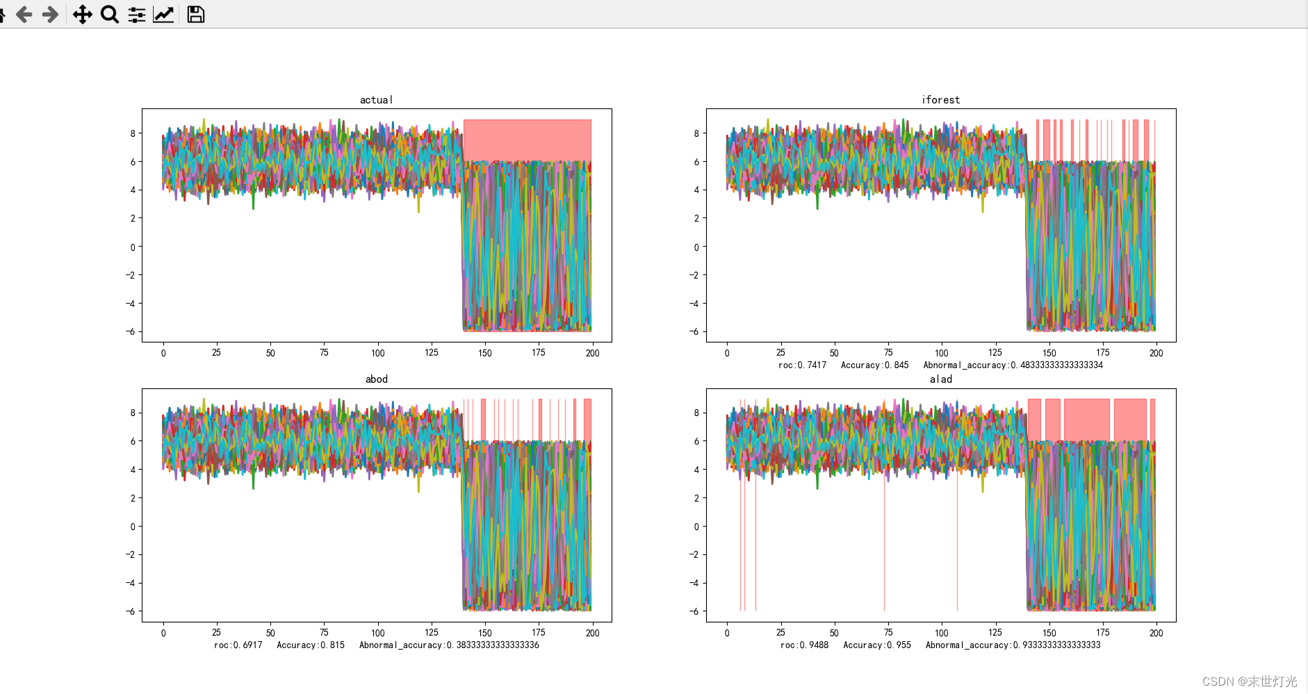
评价指标:
1. Roc曲线面积值为AUC的取值范围在0.5和1之间,AUC越接近1.0,检测方法真实性越高;等于0.5时,则真实性最低,无应用价值。
2. Accuracy参数表示针对整个测试数据集预测正确的比例,例如:
y_test = [0, 0, 0, 0, 0, 0, 1, 1, 1, 1]
y_pred = [0, 1, 0, 0, 0, 0, 0, 1, 1, 1]
其中,0代表正常数据值,1代表异常数据值,Accuracy = 8/10 = 0.8
3. Abnormal_accuracy参数表示预测出异常数据点占总异常数据的比例,例如:
y_test = [0, 0, 0, 0, 0, 0, 1, 1, 1, 1]
y_pred = [0, 1, 0, 0, 0, 0, 0, 1, 1, 1]
其中,0代表正常数据值,1代表异常数据值,Abnormal_accuracy = 3/4 = 0.75
目前测试单点异常11种方法:
整理关键数据信息:
|
方法 |
ROC |
ACC |
AB_ACC |
|
iforest |
0.7417 |
0.845 |
0.4833 |
|
abod |
0.6917 |
0.815 |
0.3833 |
|
alad |
0.9488 |
0.955 |
0.9333 |
|
auto_encoder |
1.0000 |
1.000 |
1.0000 |
|
cblof |
0.7250 |
0.835 |
0.4500 |
|
cd |
0.5000 |
0.700 |
0.0000 |
|
cof |
0.4929 |
0.690 |
0.0000 |
|
knn |
0.7000 |
0.820 |
0.4000 |
|
pca |
0.6147 |
0.785 |
0.2833 |
|
hbos |
0.6500 |
0.790 |
0.3000 |
|
lof |
0.4036 |
0.565 |
0.0000 |
扩充:
代码分享:
链接:https://pan.baidu.com/s/1vGZ98-rSLx7409039YjvqQ
提取码:pzbp
--来自百度网盘超级会员V5的分享

魔乐社区(Modelers.cn) 是一个中立、公益的人工智能社区,提供人工智能工具、模型、数据的托管、展示与应用协同服务,为人工智能开发及爱好者搭建开放的学习交流平台。社区通过理事会方式运作,由全产业链共同建设、共同运营、共同享有,推动国产AI生态繁荣发展。
更多推荐


 2
2 0
0- 0


 已为社区贡献15条内容

所有评论(0)