❤️ 🧡 💛 💚 💙 💜 🖤 🤍 🤎 💔 ❣️ 💕 💞 💓 💗 💖 💘 💝 ❤️ 🧡 💛 💚 💙 💜 🖤 🤍 🤎 💔 ❣️ 💕 💞 💓 💗 💖 💘 💝

为什么要解析特征层

在深度学习中，特征层是指神经网络中的一组层，在输入数据经过前几层后，将其分析和抽象为更高层次的特征表示。这些特征层对于网络的性能和训练结果有关键的影响。因此，在深度学习网络的训练过程中，对每一层特征层进行可视化和保存，可以帮助研究者更全面地了解网络内部的运作情况，并通过可视化结果的更新来调整网络的超参数和架构，从而提升网络的性能和训练效果。此外，特征层的可视化结果也可以帮助深度学习研究者和工程师更好地理解网络的决策过程和提高解释性。

如何可视化特征层

以ResNet系列为例，在网络训练过程中，我们找到网络定义的forward函数，如下面代码：
这段代码定义了一个基于 PyTorch 的 ResNet 模型。ResNet（残差网络）是一种在图像识别等领域广泛应用的深度神经网络架构，它通过引入残差连接解决了深层网络训练中的梯度消失和梯度爆炸问题。以下是对这段代码的详细分析：

整体结构

1. 导入模块：代码开头导入了 nn 模块，这是 PyTorch 中用于构建神经网络的核心模块。
2. 定义 ResNet 类：这是整个代码的核心，定义了 ResNet 模型的结构和前向传播逻辑。
3. 定义 resnet50 函数：用于创建一个特定配置（层数为 50 层）的 ResNet 模型实例。

ResNet 类分析
构造函数 __init__

def __init__(self,
             block,
             blocks_num,
             num_classes=10,
             include_top=True,
             groups=1,
             width_per_group=64):
    super(ResNet, self).__init__()
    self.include_top = include_top
    self.in_channel = 64
    self.groups = groups
    self.width_per_group = width_per_group
    self.conv1 = nn.Conv2d(3, self.in_channel, kernel_size=7, stride=2,
                           padding=3, bias=False)
    self.bn1 = nn.BatchNorm2d(self.in_channel)
    self.relu = nn.ReLU(inplace=True)
    self.maxpool = nn.MaxPool2d(kernel_size=3, stride=2, padding=1)
    self.layer1 = self._make_layer(block, 64, blocks_num[0])
    self.layer2 = self._make_layer(block, 128, blocks_num[1], stride=2)
    self.layer3 = self._make_layer(block, 256, blocks_num[2], stride=2)
    self.layer4 = self._make_layer(block, 512, blocks_num[3], stride=2)
    if self.include_top:
        self.avgpool = nn.AdaptiveAvgPool2d((1, 1))
        self.fc = nn.Linear(512 * block.expansion, num_classes)
    for m in self.modules():
        if isinstance(m, nn.Conv2d):
            nn.init.kaiming_normal_(m.weight, mode='fan_out', nonlinearity='relu')

1. 参数说明：
   • block：用于构建 ResNet 层的基本模块，通常是 Bottleneck 或 BasicBlock。
   • blocks_num：一个列表，指定每个 ResNet 层中 block 的数量。
   • num_classes：分类任务的类别数，默认为 10。
   • include_top：是否包含最后的全连接层进行分类，默认为 True。
   • groups：分组卷积的组数，默认为 1。
   • width_per_group：每组卷积的通道数，默认为 64。
2. 初始化成员变量：
   • self.include_top：是否包含顶层全连接层的标志。
   • self.in_channel：输入通道数，初始值为 64。
   • self.groups：分组卷积的组数。
   • self.width_per_group：每组卷积的通道数。
3. 构建网络层：
   • self.conv1：第一个卷积层，输入通道为 3（RGB 图像），输出通道为 64，卷积核大小为 7x7，步长为 2，填充为 3。
   • self.bn1：批归一化层，对 conv1 的输出进行归一化。
   • self.relu：ReLU 激活函数。
   • self.maxpool：最大池化层，核大小为 3x3，步长为 2，填充为 1。
   • self.layer1、self.layer2、self.layer3、self.layer4：通过 _make_layer 方法构建的 ResNet 层。
   • 如果 include_top 为 True，则添加自适应平均池化层 self.avgpool 和全连接层 self.fc。
4. 初始化卷积层权重：使用 kaiming_normal_ 方法初始化卷积层的权重。

_make_layer 方法

def _make_layer(self, block, channel, block_num, stride=1):
    downsample = None
    if stride!= 1 or self.in_channel!= channel * block.expansion:
        downsample = nn.Sequential(
            nn.Conv2d(self.in_channel, channel * block.expansion, kernel_size=1, stride=stride, bias=False),
            nn.BatchNorm2d(channel * block.expansion))
    layers = []
    layers.append(block(self.in_channel,
                        channel,
                        downsample=downsample,
                        stride=stride,
                        groups=self.groups,
                        width_per_group=self.width_per_group))
    self.in_channel = channel * block.expansion
    for _ in range(1, block_num):
        layers.append(block(self.in_channel,
                            channel,
                            groups=self.groups,
                            width_per_group=self.width_per_group))
    return nn.Sequential(*layers)

1. 参数说明：
   • block：基本模块。
   • channel：该层的输出通道数。
   • block_num：该层中 block 的数量。
   • stride：步长，默认为 1。
2. 构建下采样层：如果步长不为 1 或者输入通道数与输出通道数不匹配，则创建一个下采样层 downsample，用于调整输入的维度。
3. 构建 ResNet 层：
   • 首先添加一个带有下采样（如果需要）的 block。
   • 然后根据 block_num 添加多个 block。
   • 最后将这些 block 组合成一个顺序模块 nn.Sequential。

forward 方法

def forward(self, x):
    x = self.conv1(x)
    x = self.bn1(x)
    x = self.relu(x)
    x = self.maxpool(x)
    x = self.layer1(x)
    x = self.layer2(x)
    x = self.layer3(x)
    x = self.layer4(x)
    if self.include_top:
        x = self.avgpool(x)
        x = torch.flatten(x, 1)
        x = self.fc(x)
    return x

1. 定义了模型的前向传播逻辑。
2. 输入数据 x 依次经过卷积层、批归一化层、激活函数、最大池化层和各个 ResNet 层。
3. 如果 include_top 为 True，则对输出进行自适应平均池化、展平，并通过全连接层进行分类。

resnet50 函数

def resnet50(num_classes=1000, include_top=True, plot_fm=False, name=""):
    return ResNet(Bottleneck, [3, 4, 6, 3], num_classes=num_classes, include_top=include_top, plot_fm=plot_fm, name=name)

1. 参数说明：
   • num_classes：分类任务的类别数，默认为 1000。
   • include_top：是否包含最后的全连接层进行分类，默认为 True。
   • plot_fm：未在代码中使用，推测可能用于绘制特征图。
   • name：未在代码中使用，可能用于命名模型。
2. 返回一个层数为 50 层的 ResNet 模型实例，使用 Bottleneck 模块，blocks_num 为 [3, 4, 6, 3]。

这段代码实现了一个通用的 ResNet 模型，并提供了创建 50 层 ResNet 模型的便捷方法。通过调整参数，可以灵活地应用于不同的图像分类任务。代码结构清晰，遵循了 PyTorch 的标准编程规范。需要注意的是，代码中部分参数（如 plot_fm 和 name）未在当前代码中得到实际应用，可能需要根据具体需求进一步扩展。同时，Bottleneck 模块未在提供的代码中定义，需要确保在使用时已经正确定义。

---

这个代码展示了resnet网络整体架构
在训练阶段我们可以加载模型（创建优化器之前）

model = resnet50()
if pretrained:
    # 加载预训练权重文件
    #model.load_state_dict(torch.load('预训练权重文件路径'))
    pass
model.fc = nn.Linear(model.fc.in_features, num_classes)
criterion = nn.CrossEntropyLoss()

知道了整体网络架构之后，我们可以在网络结构中加入可视化特征的代码，如下所示

import time
import matplotlib.pyplot as plt
import numpy as np


def draw_features(width,height,x,savename):
    tic=time.time()
    fig = plt.figure(figsize=(16, 16))
    fig.subplots_adjust(left=0.05, right=0.95, bottom=0.05, top=0.95, wspace=0.05, hspace=0.05)
    for i in range(width*height):
        plt.subplot(height,width, i + 1)
        plt.axis('off')
        # plt.tight_layout()
        img = x[0, i, :, :]
        pmin = np.min(img)
        pmax = np.max(img)
        img = (img - pmin) / (pmax - pmin + 0.000001)
        plt.imshow(img, cmap='gray')
        print("{}/{}".format(i,width*height))
    fig.savefig(savename, dpi=100)
    fig.clf()
    plt.close()
    print("time:{}".format(time.time()-tic))

class ResNet(nn.Module):
    def __init__(self,
                 block,
                 blocks_num,
                 num_classes=10,  # 种类修改的地方，是几种就把这个改成几
                 include_top=True,
                 groups=1,
                 width_per_group=64,
                 plot_fm=False,name=""): # plot_fm控制是否要绘制特征图，name控制保存文件的名字
        super(ResNet, self).__init__()
        self.plot_fm = plot_fm
        self.savepath='data/resultck/feature_map_save_{}'.format(name) # 创建保存特征图的位置
        os.makedirs(self.savepath, exist_ok=True)
        self.include_top = include_top
        self.in_channel = 64
        self.groups = groups
        self.width_per_group = width_per_group
        self.conv1 = nn.Conv2d(3, self.in_channel, kernel_size=7, stride=2,
                               padding=3, bias=False)
        self.bn1 = nn.BatchNorm2d(self.in_channel)
        self.relu = nn.ReLU(inplace=True)
        self.maxpool = nn.MaxPool2d(kernel_size=3, stride=2, padding=1)
        self.layer1 = self._make_layer(block, 64, blocks_num[0])
        self.layer2 = self._make_layer(block, 128, blocks_num[1], stride=2)
        self.layer3 = self._make_layer(block, 256, blocks_num[2], stride=2)
        self.layer4 = self._make_layer(block, 512, blocks_num[3], stride=2)
        if self.include_top:
            self.avgpool = nn.AdaptiveAvgPool2d((1, 1))  # output size = (1, 1)
            self.fc = nn.Linear(512 * block.expansion, num_classes)
        for m in self.modules():
            if isinstance(m, nn.Conv2d):
                nn.init.kaiming_normal_(m.weight, mode='fan_out', nonlinearity='relu')

    def _make_layer(self, block, channel, block_num, stride=1):
        downsample = None
        if stride != 1 or self.in_channel != channel * block.expansion:
            downsample = nn.Sequential(
                nn.Conv2d(self.in_channel, channel * block.expansion, kernel_size=1, stride=stride, bias=False),
                nn.BatchNorm2d(channel * block.expansion))
        layers = []
        layers.append(block(self.in_channel,
                            channel,
                            downsample=downsample,
                            stride=stride,
                            groups=self.groups,
                            width_per_group=self.width_per_group))
        self.in_channel = channel * block.expansion
        for _ in range(1, block_num):
            layers.append(block(self.in_channel,
                                channel,
                                groups=self.groups,
                                width_per_group=self.width_per_group))
        return nn.Sequential(*layers)

    def forward(self, x):
        if self.plot_fm:
            x = self.conv1(x)
            draw_features(8,8,x.cpu().detach().numpy(),"{}/f1_conv1.png".format(self.savepath)) # 绘制第一个卷积层所有通道的可视化情况
            print("{}/f1_conv1.png".format(self.savepath))
            x = self.bn1(x)
            draw_features(8, 8, x.cpu().detach().numpy(),"{}/f2_bn1.png".format(self.savepath))
            print("{}/f2_bn1.png".format(self.savepath))
            x = self.relu(x)
            draw_features(8, 8, x.cpu().detach().numpy(),"{}/f3_relu.png".format(self.savepath))
            print("{}/f3_relu.png".format(self.savepath))
            x = self.maxpool(x)
            draw_features(8, 8, x.cpu().detach().numpy(),"{}/f4_maxpool.png".format(self.savepath))
            print("{}/f4_maxpool.png".format(self.savepath))
            x = self.layer1(x)
            draw_features(16, 16, x.cpu().detach().numpy(), "{}/f5_layer1.png".format(self.savepath))
            print("{}/f5_layer1.png".format(self.savepath))
            x = self.layer2(x)
            draw_features(16, 32, x.cpu().detach().numpy(), "{}/f6_layer2.png".format(self.savepath))
            print("{}/f6_layer2.png".format(self.savepath))

            x = self.layer3(x)
            draw_features(32, 32, x.cpu().detach().numpy(), "{}/f7_layer3.png".format(self.savepath))
            print("{}/f7_layer3.png".format(self.savepath))

            x = self.layer4(x)
            draw_features(32, 32, x.cpu().detach().numpy()[:, 0:1024, :, :], "{}/f8_layer4.png".format(self.savepath))
            print("{}/f8_layer4.png".format(self.savepath))

            if self.include_top:
                x = self.avgpool(x)
                plt.plot(np.linspace(1, 2048, 2048), x.cpu().detach().numpy()[0, :, 0, 0])
                plt.savefig("{}/f9_avgpool.png".format(self.savepath))
                plt.clf()
                plt.close()
                x = torch.flatten(x, 1)
                x = self.fc(x)
        else:
            x = self.conv1(x)
            x = self.bn1(x)
            x = self.relu(x)
            x = self.maxpool(x)
            x = self.layer1(x)
            x = self.layer2(x)
            x = self.layer3(x)
            x = self.layer4(x)
            if self.include_top:
                x = self.avgpool(x)
                x = torch.flatten(x, 1)
                x = self.fc(x)
        return x
def resnet50(num_classes=1000, include_top=True, plot_fm=False, name=""):
    # https://download.pytorch.org/models/resnet50-19c8e357.pth
    return ResNet(Bottleneck, [3, 4, 6, 3], num_classes=num_classes, include_top=include_top, plot_fm=plot_fm, name=name)

if modelName == "resnet50":
    model = resnet50(plot_fm=plot_fm,name=modelName)
    if pretrained:
        # 加载预训练权重文件
        #model.load_state_dict(torch.load('预训练权重文件路径'))
        pass

注意
1. draw_features(8,8,x.cpu()…；这里的8,8意思是这里的通道数是64，也就是8*8。如果不清楚可以通过 print(x.cpu().detach().numpy().shape)查看
2. draw_features(32, 32, x.cpu().detach().numpy()[:, 0:1024, :, :], “{}/f8_layer4.png”.format(self.savepath))这里的1024表示最大通道数。

可视化结果如何

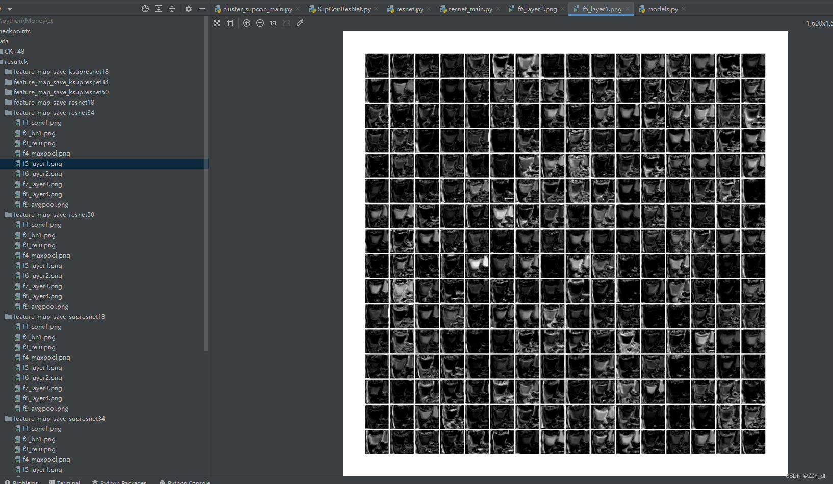
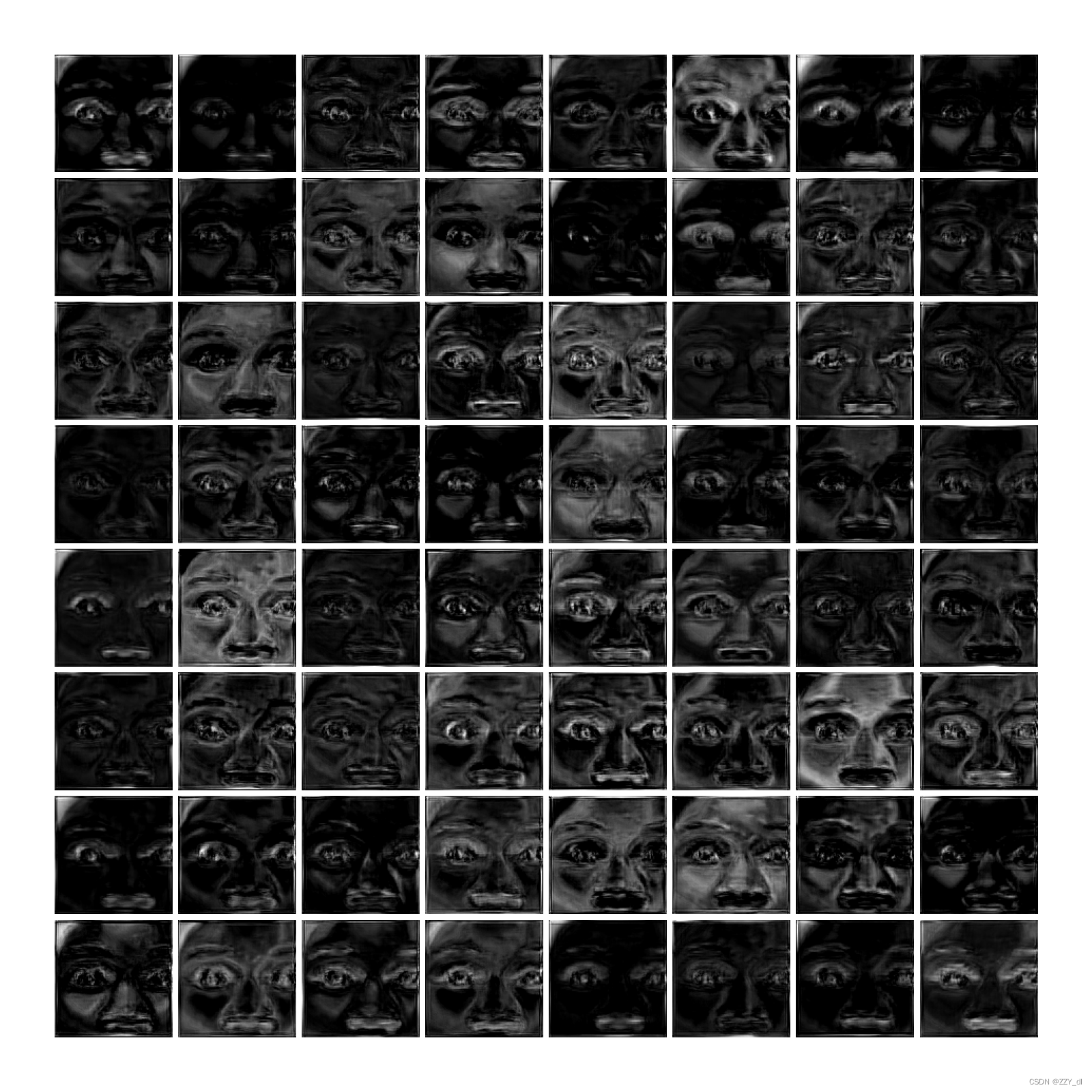
通过这样可视化，你可以清楚的看到每层特征的处理情况，以及对比不同网络下不同层的特征训练情况，通过对比可以发现哪种方法更有效。新的特征可视化情况会覆盖原始的特征可视化图，如果要在网页上实时显示，可以利用tensorboard工具来解决。可参考这篇博客：链接
非常感谢您的阅读！如果您觉得这篇文章对您有帮助，请点赞支持，您的支持是我写作的最大动力！同时，欢迎关注我的博客，我将持续分享更多深度学习、计算机视觉等方面的内容！
❤️ 🧡 💛 💚 💙 💜 🖤 🤍 🤎 💔 ❣️ 💕 💞 💓 💗 💖 💘 💝 ❤️ 🧡 💛 💚 💙 💜 🖤 🤍 🤎 💔 ❣️ 💕 💞 💓 💗 💖 💘 💝