P18深度学习软件

GPU相比CPU并行计算能力很强，非常适合做矩阵乘法，点积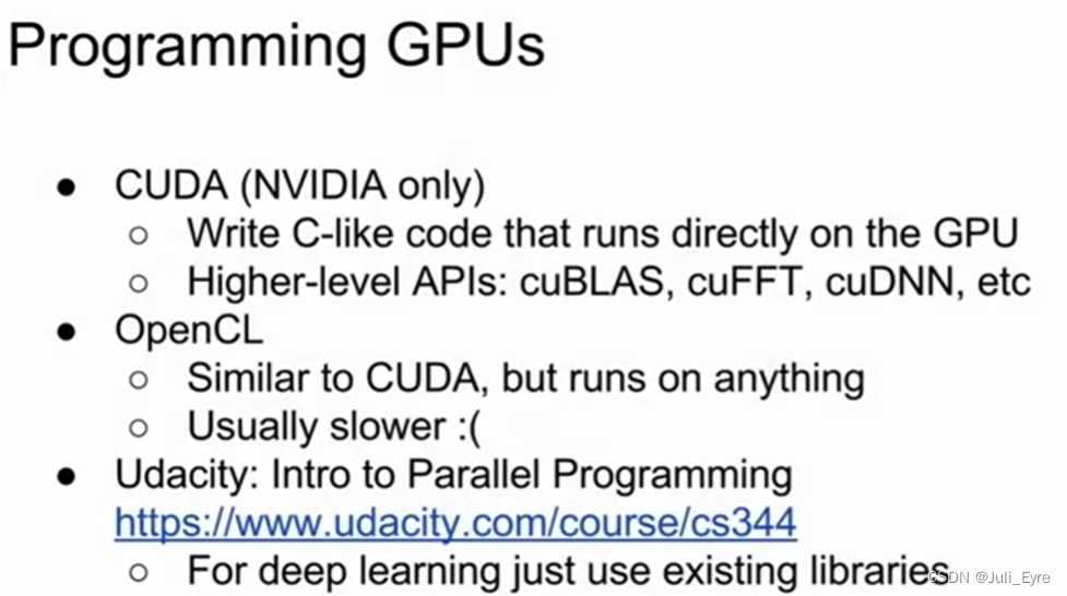

cuDNN is faster than unoptimized CUDA(大约是2-3倍，不过大多数项目都不需要用到自己写cuda)

深度学习框架已经为我们做了这事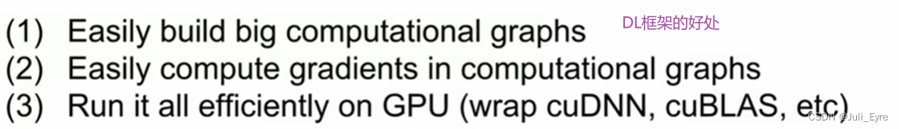

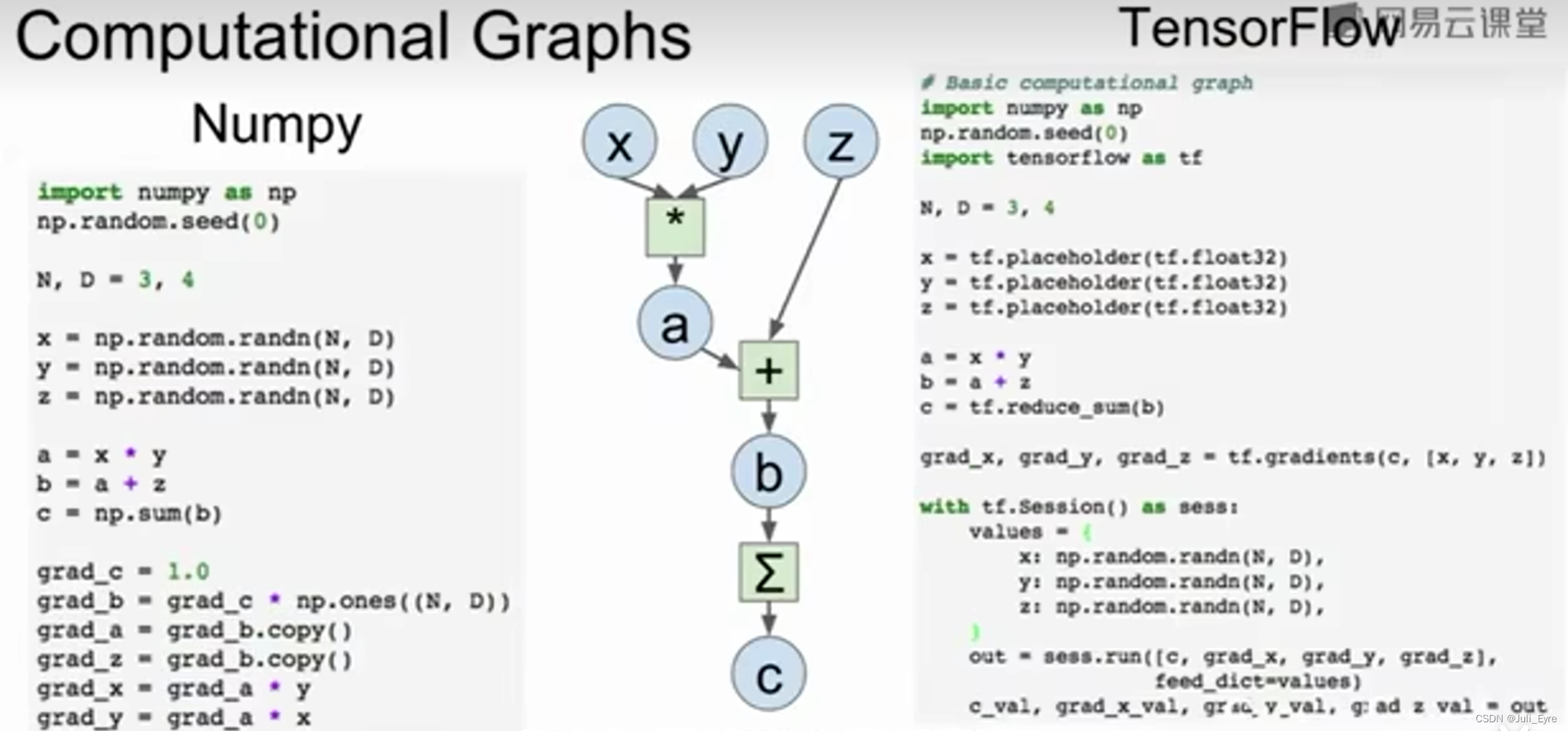
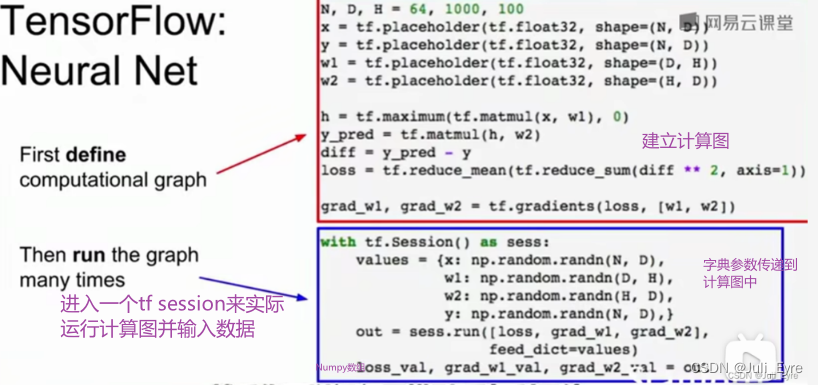
上述写法不高效，需要在Numpy和tensorflow间复制数据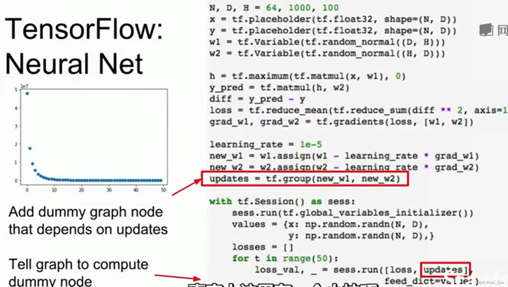

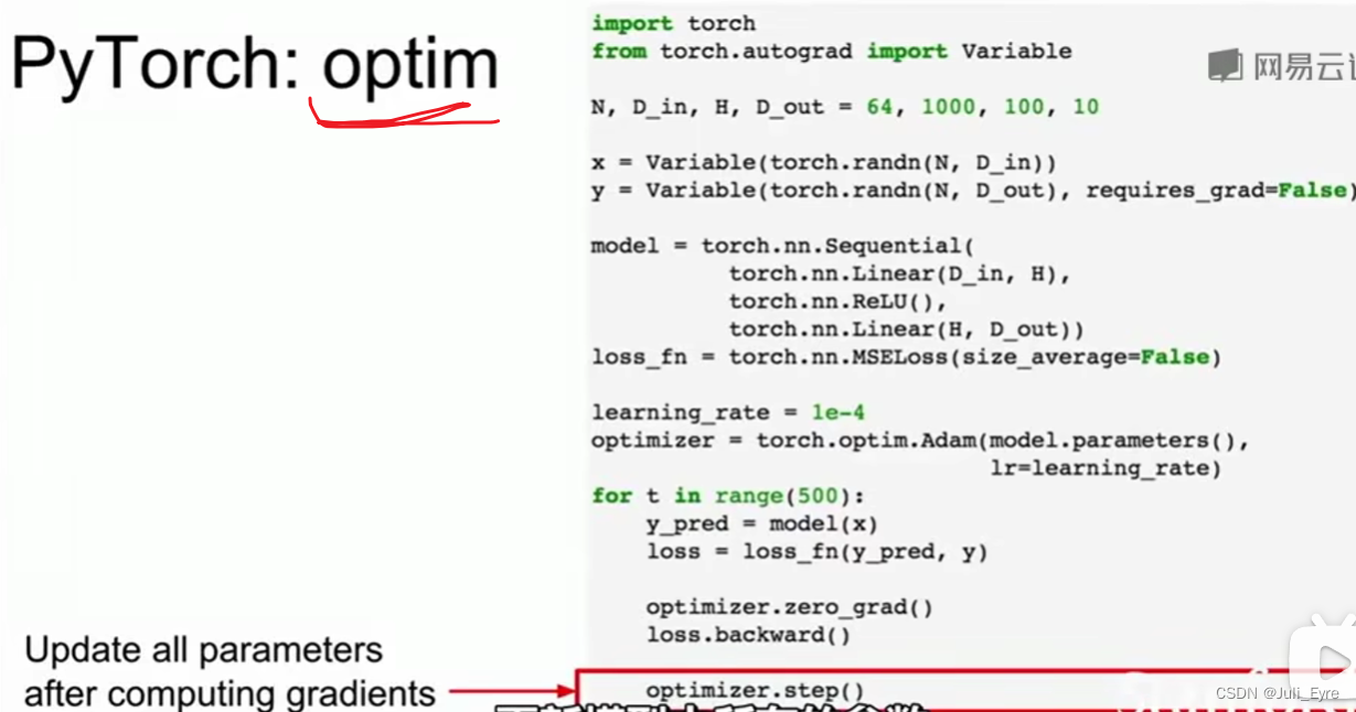
x, y是minibatch中的数据，每次都会change，因此通常没必要放进计算图中。但是必须把w1, w2, update
放进去。相当于添加了一个dummy node，当我们更新时，使用了更新的数据（updates depends on these assign operations, assign operations live inside计算图中，all inside GPU memory，而不需要把更新数据从图中拷贝出来）
*loss是一个值，updates是NULL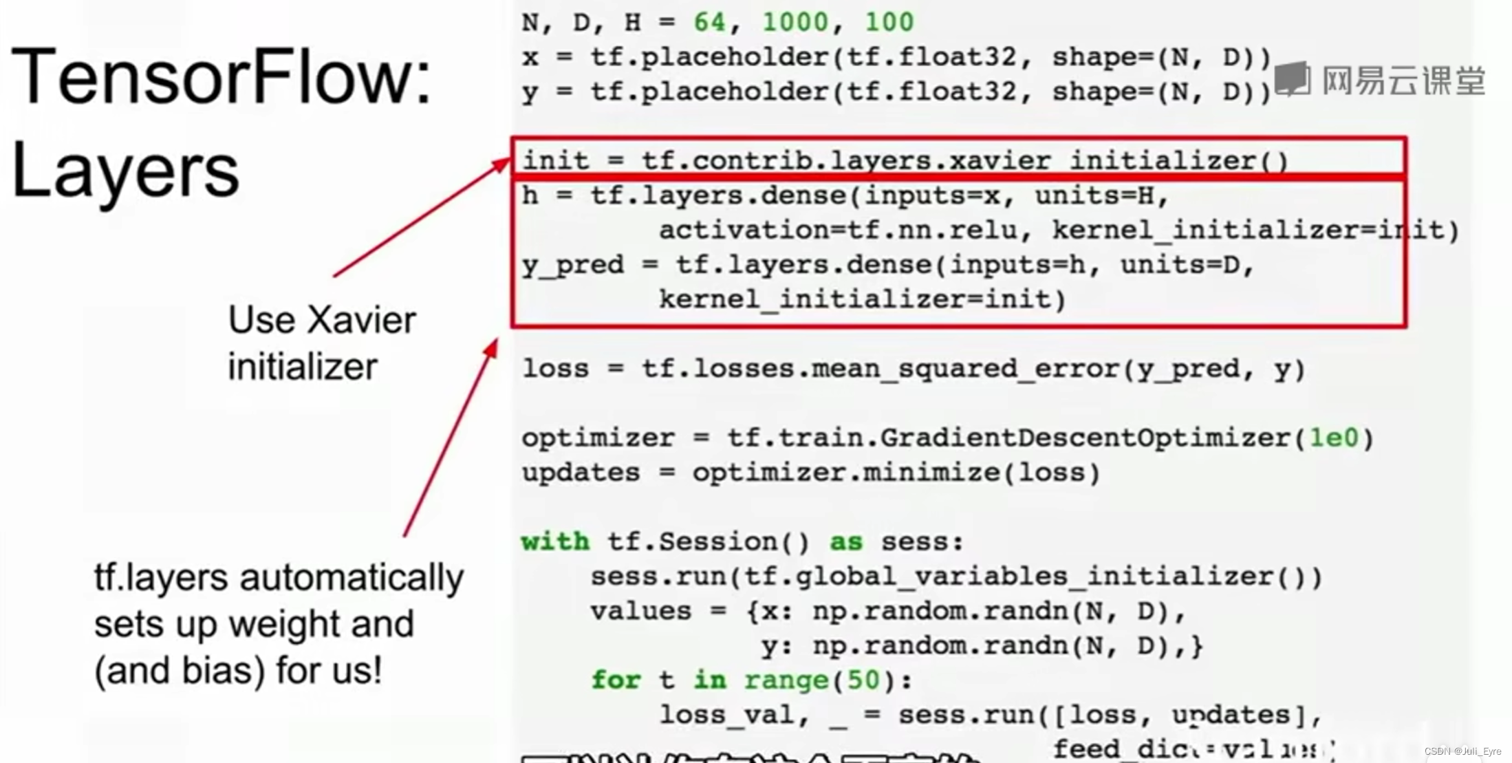

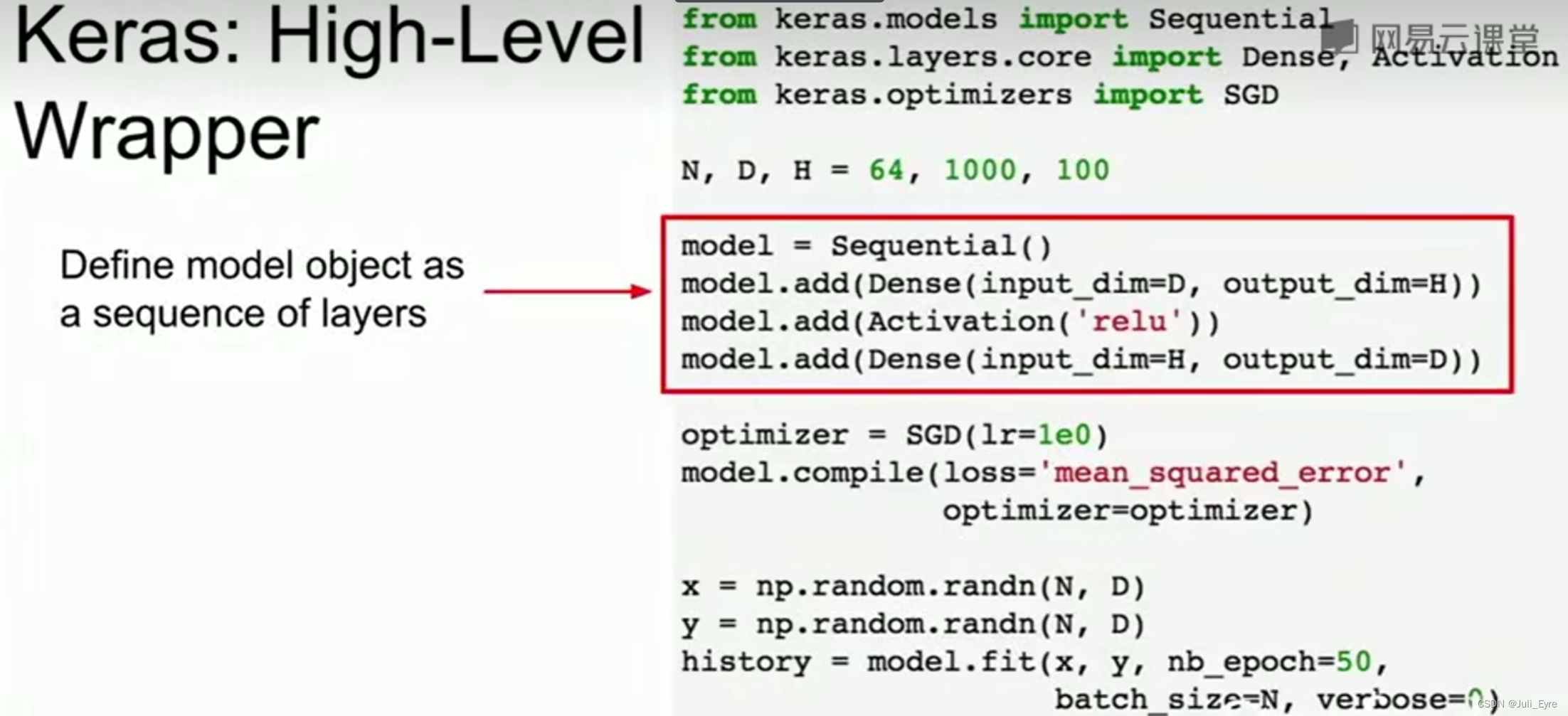
Keras基于TensorFlow的，model.fit就完成了训练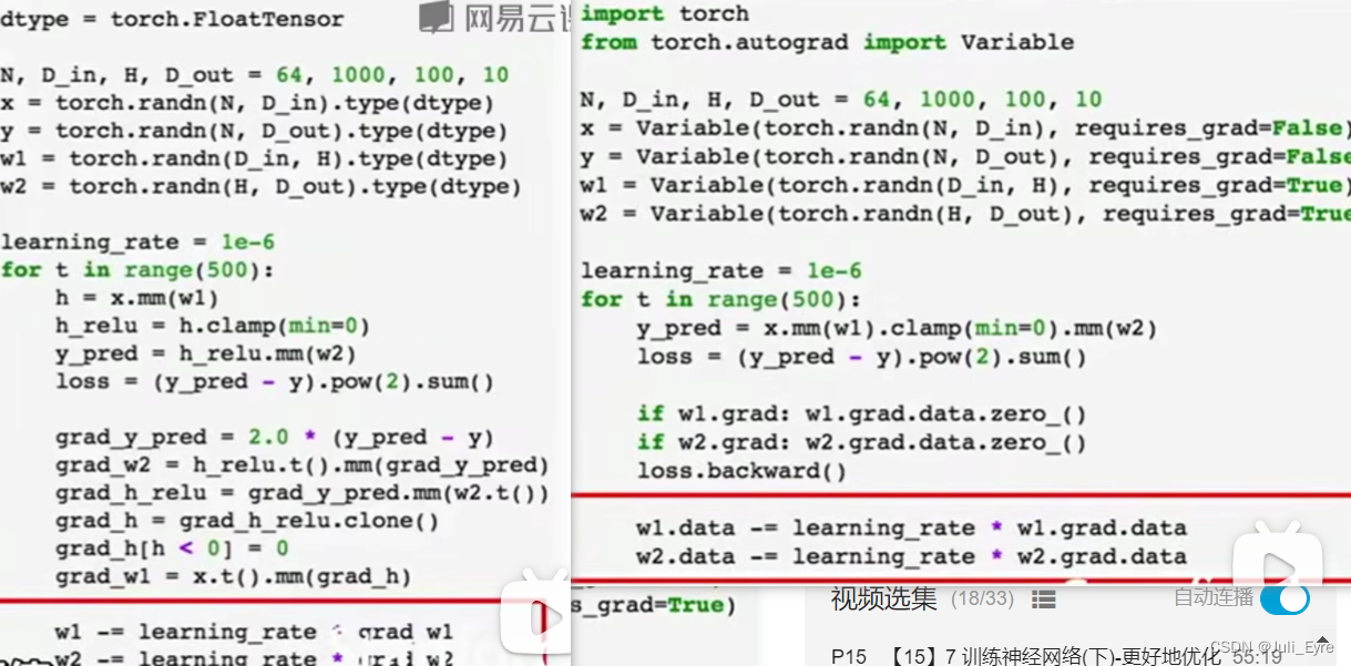

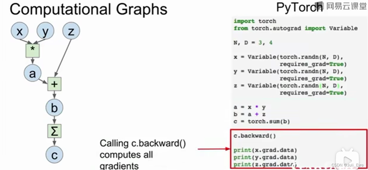
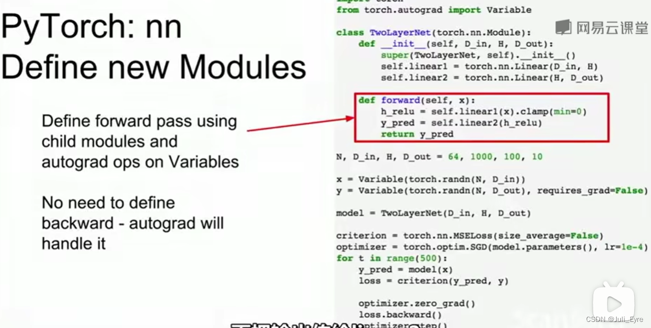
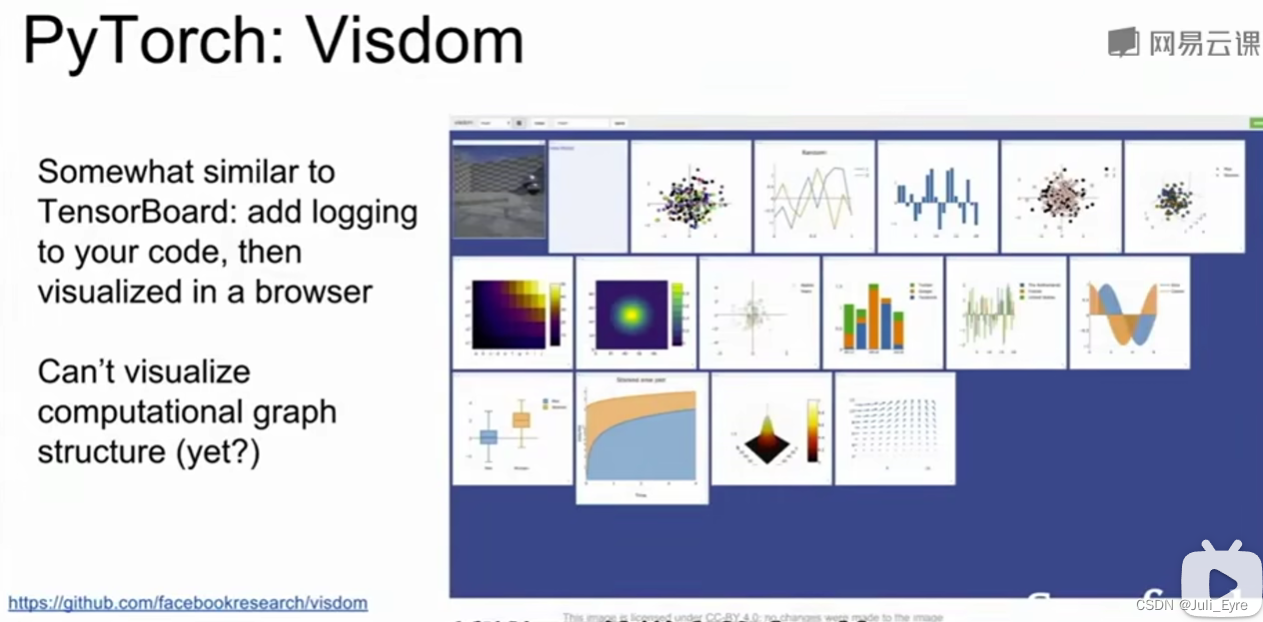
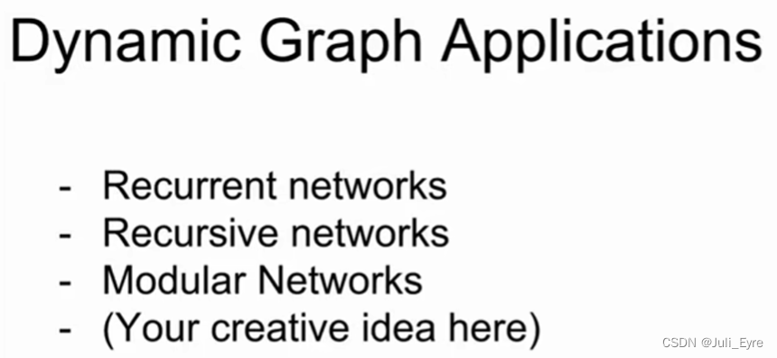
pytorch中的Tensor==Numpy+GPU，每次前向传播时都需要构造一个计算图（是动态图）

Define your own autograd functions by writing forward and backward for Tensors (similar to modularlayers):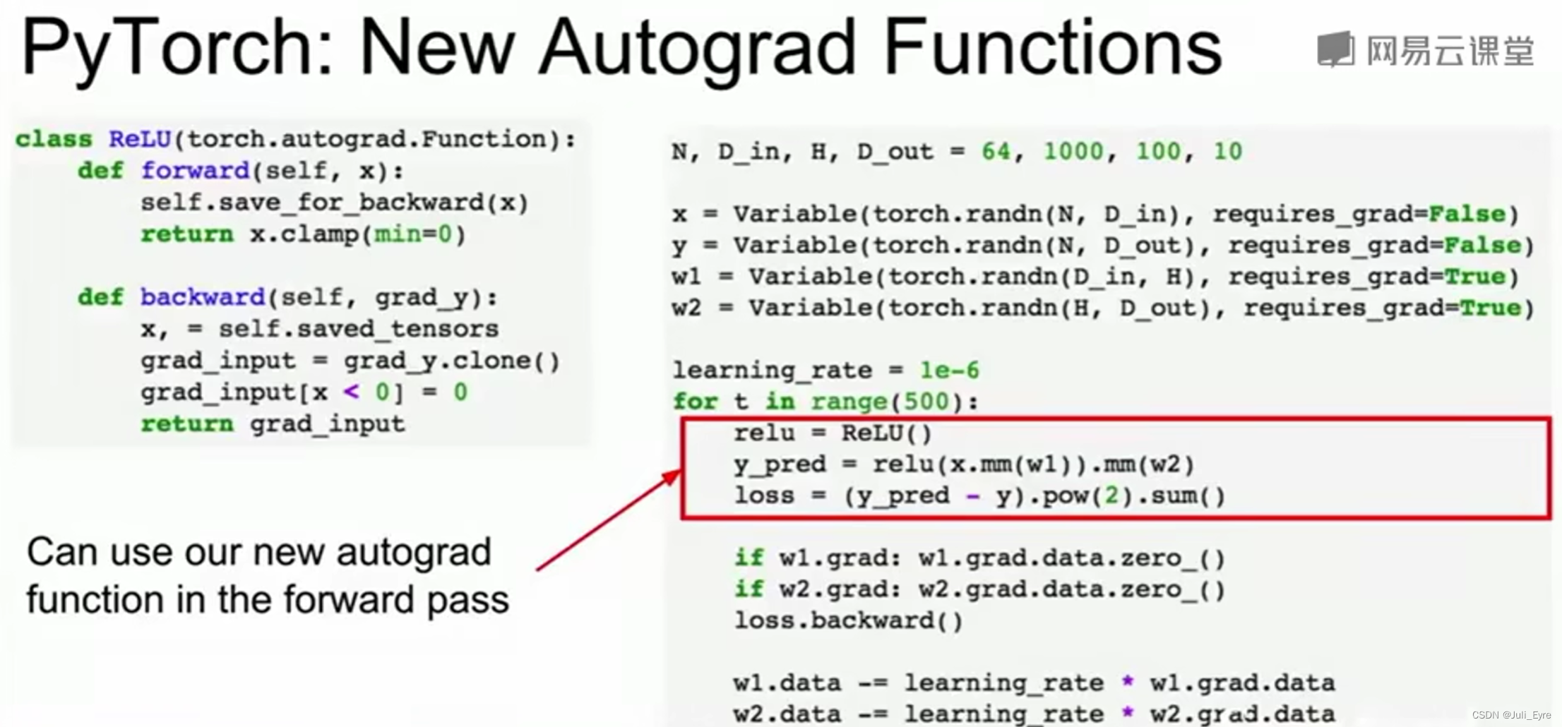







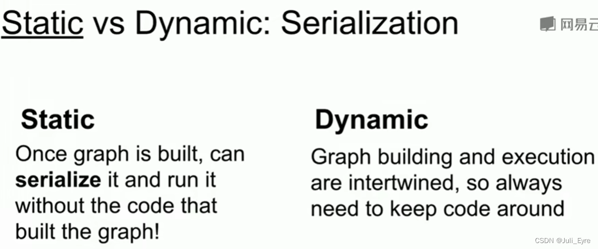
Tensorflow是静态图，建一次，然后不停地复用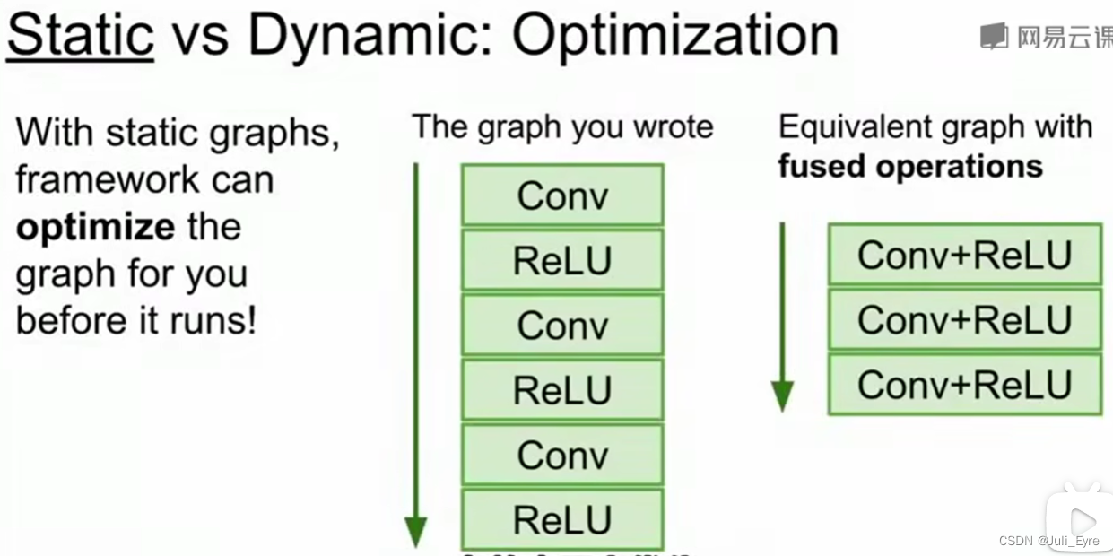

import torch
import torch.nn as nn
import torch.optim as optim
from torch.utils.data import DataLoader
from torch.utils.data import sampler

import torchvision.datasets as dset
import torchvision.transforms as T

import numpy as np

USE_GPU = True
dtype = torch.float32 # We will be using float throughout this tutorial.

if USE_GPU and torch.cuda.is_available():
    device = torch.device('cuda')
else:
    device = torch.device('cpu')

NUM_TRAIN = 49000

# The torchvision.transforms package provides tools for preprocessing data
# and for performing data augmentation; here we set up a transform to
# preprocess the data by subtracting the mean RGB value and dividing by the
# standard deviation of each RGB value; we've hardcoded the mean and std.
transform = T.Compose([
                T.ToTensor(),
                T.Normalize((0.4914, 0.4822, 0.4465), (0.2023, 0.1994, 0.2010))
            ])

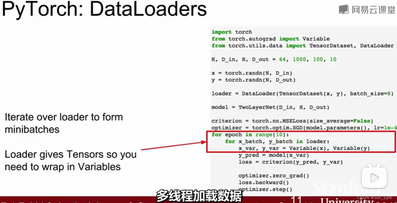
# Datasets load training examples one at a time, so we wrap each Dataset in a DataLoader
# which iterates through the Dataset and forms minibatches. 
cifar10_train = dset.CIFAR10('./cs231n/datasets', train=True, download=True,
                             transform=transform)
loader_train = DataLoader(cifar10_train, batch_size=64, 
                          sampler=sampler.SubsetRandomSampler(range(NUM_TRAIN)))

cifar10_val = dset.CIFAR10('./cs231n/datasets', train=True, download=True,
                           transform=transform)
loader_val = DataLoader(cifar10_val, batch_size=64, 
                        sampler=sampler.SubsetRandomSampler(range(NUM_TRAIN, 50000)))

cifar10_test = dset.CIFAR10('./cs231n/datasets', train=False, download=True, 
                            transform=transform)
loader_test = DataLoader(cifar10_test, batch_size=64)

import torch.nn.functional as F  # useful stateless functions

def two_layer_fc(x, params):
    """
    the architecture is: NN is fully connected -> ReLU -> fully connected layer.
   
    The input to the network will be a minibatch of data, of shape
    (N, d1, ..., dM) where d1 * ... * dM = D. The hidden layer will have H units,
    and the output layer will produce scores for C classes.
    
    Inputs:
    - x: A PyTorch Tensor of shape (N, d1, ..., dM) giving a minibatch of
      input data.
    - params: A list [w1, w2] of PyTorch Tensors giving weights for the network;
      w1 has shape (D, H) and w2 has shape (H, C).
    
    Returns:
    - scores: A PyTorch Tensor of shape (N, C) giving classification scores for
      the input data x.
    """
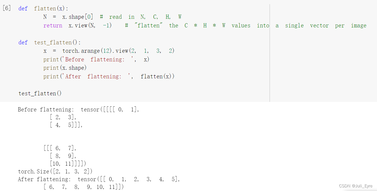
    # first we flatten the image
    # "flatten" the C * H * W values into a single vector per image
    x = flatten(x)  # shape: [batch_size, C x H x W]
    
    w1, w2 = params
    x = F.relu(x.mm(w1))
    x = x.mm(w2)
    return x

def three_layer_convnet(x, params):
    """
    a three-layer convolutional network: convolutional-convolutional-fc
    - x: A PyTorch Tensor of shape (N, 3, H, W) giving a minibatch of images
    Returns:
    - scores: PyTorch Tensor of shape (N, C) giving classification scores for x
    """
    conv_w1, conv_b1, conv_w2, conv_b2, fc_w, fc_b = params
    scores = None

    l1=F.relu_(F.conv2d(x,conv_w1,conv_b1,padding=2))
    l2=F.relu_(F.conv2d(l1,conv_w2,conv_b2,padding=1))
    scores=F.linear(flatten(l2),fc_w.T,fc_b)

    return scores

Module API: Two-Layer Network
Here is a concrete example of a 2-layer fully connected network:

class ThreeLayerConvNet(nn.Module):
    def __init__(self, in_channel, channel_1, channel_2, num_classes):
        super().__init__()
        self.conv1 = nn.Conv2d(in_channel, channel_1, 5, padding=2)
        nn.init.kaiming_normal_(self.conv1.weight)
        self.conv2 = nn.Conv2d(channel_1, channel_2, 3, padding=1)
        nn.init.kaiming_normal_(self.conv2.weight)
        self.fc = nn.Linear(channel_2*32*32, num_classes)
        nn.init.kaiming_normal_(self.fc.weight)

    def forward(self, x):
        scores = None
        # 只能使用__init__中定义的层
        c1 = F.relu(self.conv1(x))
        c2 = F.relu(self.conv2(c1))
        scores = self.fc(flatten(c2))
        return scores


def test_ThreeLayerConvNet():
    x = torch.zeros((64, 3, 32, 32), dtype=dtype)  # minibatch size 64, image size [3, 32, 32]
    model = ThreeLayerConvNet(in_channel=3, channel_1=12, channel_2=8, num_classes=10)
    scores = model(x)

def check_accuracy_part34(loader, model):
    if loader.dataset.train:
        print('Checking accuracy on validation set')
    else:
        print('Checking accuracy on test set')   
    num_correct = 0
    num_samples = 0
    model.eval()  # set model to evaluation mode
    with torch.no_grad():
        for x, y in loader:
            x = x.to(device=device, dtype=dtype)  # move to device, e.g. GPU
            y = y.to(device=device, dtype=torch.long)
            scores = model(x)
            _, preds = scores.max(1)
            num_correct += (preds == y).sum()
            num_samples += preds.size(0)
        acc = float(num_correct) / num_samples
        print('Got %d / %d correct (%.2f)' % (num_correct, num_samples, 100 * acc))

def train_part34(model, optimizer, epochs=1):
    model = model.to(device=device)  # move the model parameters to CPU/GPU
    for e in range(epochs):
        for t, (x, y) in enumerate(loader_train):
            model.train()  # put model to training mode
            x = x.to(device=device, dtype=dtype)  # move to device, e.g. GPU
            y = y.to(device=device, dtype=torch.long)

            scores = model(x)
            loss = F.cross_entropy(scores, y)

            # Zero out all of the gradients for the variables which the optimizer
            # will update.
            optimizer.zero_grad()

            # This is the backwards pass: compute the gradient of the loss with
            # respect to each  parameter of the model.
            loss.backward()

            # Actually update the parameters of the model using the gradients
            # computed by the backwards pass.
            optimizer.step()

            if t % print_every == 0:
                print('Iteration %d, loss = %.4f' % (t, loss.item()))
                check_accuracy_part34(loader_val, model)
                print()
                
# We need to wrap `flatten` function in a module in order to stack it
# in nn.Sequential
class Flatten(nn.Module):
    def forward(self, x):
        return flatten(x)

hidden_layer_size = 4000
learning_rate = 1e-2

model = nn.Sequential(
    Flatten(),
    nn.Linear(3 * 32 * 32, hidden_layer_size),
    nn.ReLU(),
    nn.Linear(hidden_layer_size, 10),
)

# you can use Nesterov momentum in optim.SGD
optimizer = optim.SGD(model.parameters(), lr=learning_rate,
                     momentum=0.9, nesterov=True)

train_part34(model, optimizer)

识别与分割

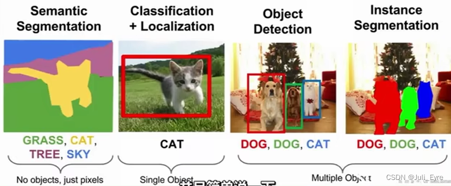
P25语义分割：对每个像素进行分类，不会区分同类物体–>Instance Segmentation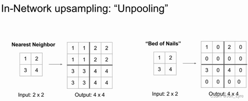


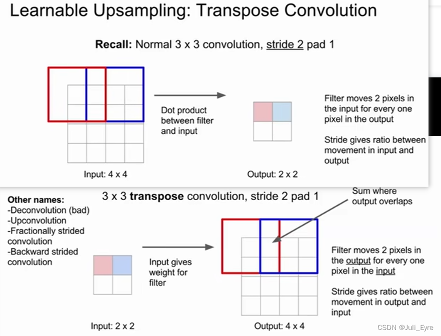
strided convolution一种downsampling方法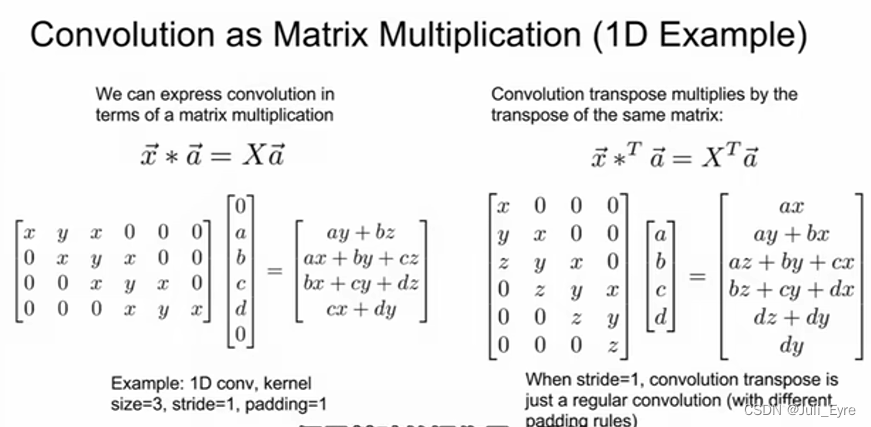

P23定位：multi-loss: 加权系数的选择，可以通过用性能矩阵做交叉验证而不仅仅是loss值
P24 object detection: 与定位相比，是不知道对象的数量的

1. region-based methods: 一个常用的候选区域方法就是目标检测。
   先使用候选区域网络找到物体可能存在的备选区域（Regions of Interest, ROI），然后再利用卷积神经网络对备选区域进行分类。

• 对备选区域做切分，使之大小一样
• 回归预测补偿修正边界值（备选区域的划分并不完美）
  RCNN也是这样做的，是监督学习

2. 不是基于候选框的，而是作为回归问题处理的
   Instance Segmentation: 逐像素的分割

可视化与理解

可视化卷积核的权重：为了理解卷积核在找什么（内积最大化的是和所用模板相匹配的）

对抗样本

不是noise，噪音相比对抗样本对网络的影响是很小的
显示器是8位，模型参数是32位float，我们仅改变另24位
gradient on the input images
原因：模型线性程度的假设过高造成的，不是线性的偏偏推断成线性的就会产生这样的对抗样本（如FGSM）；只要能找到一个和梯度方向形成很大内积的方向，沿着个方向移动一点，就可以欺骗神经网络。

在高维空间中选一个参考向量，再选一个随机向量。平均意义上讲，他两的内积为0，随机向量对损失函数是没有影响的（可以通过对损失函数进行一阶泰勒展开分析随机向量的影响）。但是用对抗样本最大化it。

对抗子空间的维数实际代表了由一个随机噪声找到对抗样本的容易程度。对抗子空间的维数和迁移性质息息相关。对抗子空间越大，在不同模型之间的迁移越容易。（子空间是随机的）
不同的模型往往在同样的对抗样本上犯错。
shallow RBF model能很好的抵抗对抗扰动

model-based optimization

同样的扰动可能用在不同的模型或不同的干净样本上，因为对抗子空间only about 50维，即使输入空间是3000维的。
不能在softmax前对最后一层做扰动。（因为最后一层是线性的，不可能抵挡扰动。在这层做对抗训练，通常会破坏整个过程）
对抗训练非常需要数据。