头歌机器学习(2)
【代码】头歌机器学习(2)
·
本文仅供机器学习参考
1、逻辑回归
1、逻辑回归核心思想
#encoding=utf8
#encoding=utf8
import numpy as np

def sigmoid(t):
    '''
    完成sigmoid函数计算
    :param t: 负无穷到正无穷的实数
    :return: 转换后的概率值
    :可以考虑使用np.exp()函数
    '''
    #********** Begin **********#
    return  1.0/(1+np.exp(-t))

    #********** End **********#
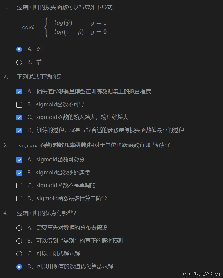
2、逻辑回归的损失函数
3、梯度下降
## -*- coding: utf-8 -*-

import numpy as np
import warnings
warnings.filterwarnings("ignore")

def gradient_descent(initial_theta,eta=0.05,n_iters=1000,epslion=1e-8):
    '''
    梯度下降
    :param initial_theta: 参数初始值,类型为float
    :param eta: 学习率,类型为float
    :param n_iters: 训练轮数,类型为int
    :param epslion: 容忍误差范围,类型为float
    :return: 训练后得到的参数
    '''
    #   请在此添加实现代码   #
    #********** Begin *********#
    theta = initial_theta
    i_iter = 0
    while i_iter < n_iters:
        gradient = 2*(theta-3)
        last_theta = theta
        theta = theta - eta*gradient
        if(abs(theta-last_theta)<epslion):
            break
        i_iter +=1
    return theta
    #********** End **********#
4、动手实现逻辑回归 - 癌细胞精准识别
# -*- coding: utf-8 -*-

import numpy as np
import warnings
warnings.filterwarnings("ignore")

def sigmoid(x):
    '''
    sigmoid函数
    :param x: 转换前的输入
    :return: 转换后的概率
    '''
    return 1/(1+np.exp(-x))


def fit(x,y,eta=1e-3,n_iters=10000):
    '''
    训练逻辑回归模型
    :param x: 训练集特征数据,类型为ndarray
    :param y: 训练集标签,类型为ndarray
    :param eta: 学习率,类型为float
    :param n_iters: 训练轮数,类型为int
    :return: 模型参数,类型为ndarray
    '''
    #   请在此添加实现代码   #
    #********** Begin *********#
    theta = np.zeros(x.shape[1])
    i_iter = 0
    while i_iter < n_iters:
        gradient = (sigmoid(x.dot(theta))-y).dot(x)
        theta = theta -eta*gradient
        i_iter += 1
    return theta
    #********** End **********#
5、手写数字识别
from sklearn.linear_model import LogisticRegression

def digit_predict(train_image, train_label, test_image):
    '''
    实现功能:训练模型并输出预测结果
    :param train_sample: 包含多条训练样本的样本集,类型为ndarray,shape为[-1, 8, 8]
    :param train_label: 包含多条训练样本标签的标签集,类型为ndarray
    :param test_sample: 包含多条测试样本的测试集,类型为ndarry
    :return: test_sample对应的预测标签
    '''

    #************* Begin ************#
    # 训练集变形
    flat_train_image = train_image.reshape((-1, 64))
    # 训练集标准化
    train_min = flat_train_image.min()
    train_max = flat_train_image.max()
    flat_train_image = (flat_train_image-train_min)/(train_max-train_min)
    # 测试集变形
    flat_test_image = test_image.reshape((-1, 64))
    # 测试集标准化
    test_min = flat_test_image.min()
    test_max = flat_test_image.max()
    flat_test_image = (flat_test_image - test_min) / (test_max - test_min)

    # 训练--预测
    rf = LogisticRegression(C=4.0)
    rf.fit(flat_train_image, train_label)
    return rf.predict(flat_test_image)
    #************* End **************#
2、决策树
1、什么是决策树

2、信息熵与信息增益
import numpy as np
def calcInfoGain(feature, label, index):
    '''
    计算信息增益
    :param feature:测试用例中字典里的feature,类型为ndarray
    :param label:测试用例中字典里的label,类型为ndarray
    :param index:测试用例中字典里的index,即feature部分特征列的索引。该索引指的是feature中第几个特征,如index:0表示使用第一个特征来计算信息增益。
    :return:信息增益,类型float
    '''

    #*********** Begin ***********#
    # 计算熵
    def calcInfoEntropy(feature, label):
        '''
        计算信息熵
        :param feature:数据集中的特征,类型为ndarray
        :param label:数据集中的标签,类型为ndarray
        :return:信息熵,类型float
        '''

        label_set = set(label)
        result = 0
        for l in label_set:
            count = 0
            for j in range(len(label)):
                if label[j] == l:
                    count += 1
            # 计算标签在数据集中出现的概率
            p = count / len(label)
            # 计算熵
            result -= p * np.log2(p)
        return result

    # 计算条件熵
    def calcHDA(feature, label, index, value):
        '''
        计算信息熵
        :param feature:数据集中的特征,类型为ndarray
        :param label:数据集中的标签,类型为ndarray
        :param index:需要使用的特征列索引,类型为int
        :param value:index所表示的特征列中需要考察的特征值,类型为int
        :return:信息熵,类型float
        '''
        count = 0
        # sub_feature和sub_label表示根据特征列和特征值分割出的子数据集中的特征和标签
        sub_feature = []
        sub_label = []
        for i in range(len(feature)):
            if feature[i][index] == value:
                count += 1
                sub_feature.append(feature[i])
                sub_label.append(label[i])
        pHA = count / len(feature)
        e = calcInfoEntropy(sub_feature, sub_label)
        return pHA * e

    base_e = calcInfoEntropy(feature, label)
    f = np.array(feature)
    # 得到指定特征列的值的集合
    f_set = set(f[:, index])
    sum_HDA = 0
    # 计算条件熵
    for value in f_set:
        sum_HDA += calcHDA(feature, label, index, value)
    # 计算信息增益
    return base_e - sum_HDA

    #*********** End *************#
3、使用ID3算法构建决策树
import numpy as np
class DecisionTree(object):
    def __init__(self):
        #决策树模型
        self.tree = {}
    def calcInfoGain(self, feature, label, index):
        '''
        计算信息增益
        :param feature:测试用例中字典里的feature,类型为ndarray
        :param label:测试用例中字典里的label,类型为ndarray
        :param index:测试用例中字典里的index,即feature部分特征列的索引。该索引指的是feature中第几个特征,如index:0表示使用第一个特征来计算信息增益。
        :return:信息增益,类型float
        '''
        # 计算熵
        def calcInfoEntropy(label):
            '''
            计算信息熵
            :param label:数据集中的标签,类型为ndarray
            :return:信息熵,类型float
            '''
            label_set = set(label)
            result = 0
            for l in label_set:
                count = 0
                for j in range(len(label)):
                    if label[j] == l:
                        count += 1
                # 计算标签在数据集中出现的概率
                p = count / len(label)
                # 计算熵
                result -= p * np.log2(p)
            return result
        # 计算条件熵
        def calcHDA(feature, label, index, value):
            '''
            计算信息熵
            :param feature:数据集中的特征,类型为ndarray
            :param label:数据集中的标签,类型为ndarray
            :param index:需要使用的特征列索引,类型为int
            :param value:index所表示的特征列中需要考察的特征值,类型为int
            :return:信息熵,类型float
            '''
            count = 0
            # sub_feature和sub_label表示根据特征列和特征值分割出的子数据集中的特征和标签
            sub_feature = []
            sub_label = []
            for i in range(len(feature)):
                if feature[i][index] == value:
                    count += 1
                    sub_feature.append(feature[i])
                    sub_label.append(label[i])
            pHA = count / len(feature)
            e = calcInfoEntropy(sub_label)
            return pHA * e
        base_e = calcInfoEntropy(label)
        f = np.array(feature)
        # 得到指定特征列的值的集合
        f_set = set(f[:, index])
        sum_HDA = 0
        # 计算条件熵
        for value in f_set:
            sum_HDA += calcHDA(feature, label, index, value)
        # 计算信息增益
        return base_e - sum_HDA
    # 获得信息增益最高的特征
    def getBestFeature(self, feature, label):
        max_infogain = 0
        best_feature = 0
        for i in range(len(feature[0])):
            infogain = self.calcInfoGain(feature, label, i)
            if infogain > max_infogain:
                max_infogain = infogain
                best_feature = i
        return best_feature
    def createTree(self, feature, label):
        # 样本里都是同一个label没必要继续分叉了
        if len(set(label)) == 1:
            return label[0]
        # 样本中只有一个特征或者所有样本的特征都一样的话就看哪个label的票数高
        if len(feature[0]) == 1 or len(np.unique(feature, axis=0)) == 1:
            vote = {}
            for l in label:
                if l in vote.keys():
                    vote[l] += 1
                else:
                    vote[l] = 1
            max_count = 0
            vote_label = None
            for k, v in vote.items():
                if v > max_count:
                    max_count = v
                    vote_label = k
            return vote_label
        # 根据信息增益拿到特征的索引
        best_feature = self.getBestFeature(feature, label)
        tree = {best_feature: {}}
        f = np.array(feature)
        # 拿到bestfeature的所有特征值
        f_set = set(f[:, best_feature])
        # 构建对应特征值的子样本集sub_feature, sub_label
        for v in f_set:
            sub_feature = []
            sub_label = []
            for i in range(len(feature)):
                if feature[i][best_feature] == v:
                    sub_feature.append(feature[i])
                    sub_label.append(label[i])
            # 递归构建决策树
            tree[best_feature][v] = self.createTree(sub_feature, sub_label)
        return tree
    def fit(self, feature, label):
        '''
        :param feature: 训练集数据,类型为ndarray
        :param label:训练集标签,类型为ndarray
        :return: None
        '''
        #************* Begin ************#
        self.tree = self.createTree(feature, label)

        #************* End **************#
    def predict(self, feature):
        '''
        :param feature:测试集数据,类型为ndarray
        :return:预测结果,如np.array([0, 1, 2, 2, 1, 0])
        '''
        #************* Begin ************#
        result = []
        def classify(tree, feature):
            if not isinstance(tree, dict):
                return tree
            t_index, t_value = list(tree.items())[0]
            f_value = feature[t_index]
            if isinstance(t_value, dict):
                classLabel = classify(tree[t_index][f_value], feature)
                return classLabel
            else:
                return t_value
        for f in feature:
            result.append(classify(self.tree, f))
        return np.array(result)
        #************* End **************#
4、信息增益率
import numpy as np
def calcInfoGain(feature, label, index):
    '''
    计算信息增益
    :param feature:测试用例中字典里的feature,类型为ndarray
    :param label:测试用例中字典里的label,类型为ndarray
    :param index:测试用例中字典里的index,即feature部分特征列的索引。该索引指的是feature中第几个特征,如index:0表示使用第一个特征来计算信息增益。
    :return:信息增益,类型float
    '''
    # 计算熵
    def calcInfoEntropy(label):
        '''
        计算信息熵
        :param label:数据集中的标签,类型为ndarray
        :return:信息熵,类型float
        '''

        label_set = set(label)
        result = 0
        for l in label_set:
            count = 0
            for j in range(len(label)):
                if label[j] == l:
                    count += 1
            # 计算标签在数据集中出现的概率
            p = count / len(label)
            # 计算熵
            result -= p * np.log2(p)
        return result

    # 计算条件熵
    def calcHDA(feature, label, index, value):
        '''
        计算信息熵
        :param feature:数据集中的特征,类型为ndarray
        :param label:数据集中的标签,类型为ndarray
        :param index:需要使用的特征列索引,类型为int
        :param value:index所表示的特征列中需要考察的特征值,类型为int
        :return:信息熵,类型float
        '''
        count = 0
        # sub_label表示根据特征列和特征值分割出的子数据集中的标签
        sub_label = []
        for i in range(len(feature)):
            if feature[i][index] == value:
                count += 1
                sub_label.append(label[i])
        pHA = count / len(feature)
        e = calcInfoEntropy(sub_label)
        return pHA * e

    base_e = calcInfoEntropy(label)
    f = np.array(feature)
    # 得到指定特征列的值的集合
    f_set = set(f[:, index])
    sum_HDA = 0
    # 计算条件熵
    for value in f_set:
        sum_HDA += calcHDA(feature, label, index, value)
    # 计算信息增益
    return base_e - sum_HDA


def calcInfoGainRatio(feature, label, index):
    '''
    计算信息增益率
    :param feature:测试用例中字典里的feature,类型为ndarray
    :param label:测试用例中字典里的label,类型为ndarray
    :param index:测试用例中字典里的index,即feature部分特征列的索引。该索引指的是feature中第几个特征,如index:0表示使用第一个特征来计算信息增益。
    :return:信息增益率,类型float
    '''

    #********* Begin *********#
    info_gain = calcInfoGain(feature, label, index)
    unique_value = list(set(feature[:, index]))
    IV = 0
    for value in unique_value:
        len_v = np.sum(feature[:, index] == value)
        IV -= (len_v/len(feature))*np.log2((len_v/len(feature)))
    return info_gain/IV

    #********* End *********#
5、基尼系数
import numpy as np
def calcGini(feature, label, index):
    '''
    计算基尼系数
    :param feature:测试用例中字典里的feature,类型为ndarray
    :param label:测试用例中字典里的label,类型为ndarray
    :param index:测试用例中字典里的index,即feature部分特征列的索引。该索引指的是feature中第几个特征,如index:0表示使用第一个特征来计算信息增益。
    :return:基尼系数,类型float
    '''

    #********* Begin *********#
    def _gini(label):
        unique_label = list(set(label))
        gini = 1
        for l in unique_label:
            p = np.sum(label == l)/len(label)
            gini -= p**2
        return gini
    unique_value = list(set(feature[:, index]))
    gini = 0
    for value in unique_value:
        len_v = np.sum(feature[:, index] == value)
        gini += (len_v/len(feature))*_gini(label[feature[:, index] == value])
    return gini
    #********* End *********#
6、预剪枝与后剪枝
import numpy as np
from copy import deepcopy
class DecisionTree(object):
    def __init__(self):
        #决策树模型
        self.tree = {}
    def calcInfoGain(self, feature, label, index):
        '''
        计算信息增益
        :param feature:测试用例中字典里的feature,类型为ndarray
        :param label:测试用例中字典里的label,类型为ndarray
        :param index:测试用例中字典里的index,即feature部分特征列的索引。该索引指的是feature中第几个特征,如index:0表示使用第一个特征来计算信息增益。
        :return:信息增益,类型float
        '''
        # 计算熵
        def calcInfoEntropy(feature, label):
            '''
            计算信息熵
            :param feature:数据集中的特征,类型为ndarray
            :param label:数据集中的标签,类型为ndarray
            :return:信息熵,类型float
            '''
            label_set = set(label)
            result = 0
            for l in label_set:
                count = 0
                for j in range(len(label)):
                    if label[j] == l:
                        count += 1
                # 计算标签在数据集中出现的概率
                p = count / len(label)
                # 计算熵
                result -= p * np.log2(p)
            return result
        # 计算条件熵
        def calcHDA(feature, label, index, value):
            '''
            计算信息熵
            :param feature:数据集中的特征,类型为ndarray
            :param label:数据集中的标签,类型为ndarray
            :param index:需要使用的特征列索引,类型为int
            :param value:index所表示的特征列中需要考察的特征值,类型为int
            :return:信息熵,类型float
            '''
            count = 0
            # sub_feature和sub_label表示根据特征列和特征值分割出的子数据集中的特征和标签
            sub_feature = []
            sub_label = []
            for i in range(len(feature)):
                if feature[i][index] == value:
                    count += 1
                    sub_feature.append(feature[i])
                    sub_label.append(label[i])
            pHA = count / len(feature)
            e = calcInfoEntropy(sub_feature, sub_label)
            return pHA * e
        base_e = calcInfoEntropy(feature, label)
        f = np.array(feature)
        # 得到指定特征列的值的集合
        f_set = set(f[:, index])
        sum_HDA = 0
        # 计算条件熵
        for value in f_set:
            sum_HDA += calcHDA(feature, label, index, value)
        # 计算信息增益
        return base_e - sum_HDA
    # 获得信息增益最高的特征
    def getBestFeature(self, feature, label):
        max_infogain = 0
        best_feature = 0
        for i in range(len(feature[0])):
            infogain = self.calcInfoGain(feature, label, i)
            if infogain > max_infogain:
                max_infogain = infogain
                best_feature = i
        return best_feature
    # 计算验证集准确率
    def calc_acc_val(self, the_tree, val_feature, val_label):
        result = []
        def classify(tree, feature):
            if not isinstance(tree, dict):
                return tree
            t_index, t_value = list(tree.items())[0]
            f_value = feature[t_index]
            if isinstance(t_value, dict):
                classLabel = classify(tree[t_index][f_value], feature)
                return classLabel
            else:
                return t_value
        for f in val_feature:
            result.append(classify(the_tree, f))
        result = np.array(result)
        return np.mean(result == val_label)
    def createTree(self, train_feature, train_label):
        # 样本里都是同一个label没必要继续分叉了
        if len(set(train_label)) == 1:
            return train_label[0]
        # 样本中只有一个特征或者所有样本的特征都一样的话就看哪个label的票数高
        if len(train_feature[0]) == 1 or len(np.unique(train_feature, axis=0)) == 1:
            vote = {}
            for l in train_label:
                if l in vote.keys():
                    vote[l] += 1
                else:
                    vote[l] = 1
            max_count = 0
            vote_label = None
            for k, v in vote.items():
                if v > max_count:
                    max_count = v
                    vote_label = k
            return vote_label
        # 根据信息增益拿到特征的索引
        best_feature = self.getBestFeature(train_feature, train_label)
        tree = {best_feature: {}}
        f = np.array(train_feature)
        # 拿到bestfeature的所有特征值
        f_set = set(f[:, best_feature])
        # 构建对应特征值的子样本集sub_feature, sub_label
        for v in f_set:
            sub_feature = []
            sub_label = []
            for i in range(len(train_feature)):
                if train_feature[i][best_feature] == v:
                    sub_feature.append(train_feature[i])
                    sub_label.append(train_label[i])
            # 递归构建决策树
            tree[best_feature][v] = self.createTree(sub_feature, sub_label)
        return tree
    # 后剪枝
    def post_cut(self, val_feature, val_label):
        # 拿到非叶子节点的数量
        def get_non_leaf_node_count(tree):
            non_leaf_node_path = []
            def dfs(tree, path, all_path):
                for k in tree.keys():
                    if isinstance(tree[k], dict):
                        path.append(k)
                        dfs(tree[k], path, all_path)
                        if len(path) > 0:
                            path.pop()
                    else:
                        all_path.append(path[:])
            dfs(tree, [], non_leaf_node_path)
            unique_non_leaf_node = []
            for path in non_leaf_node_path:
                isFind = False
                for p in unique_non_leaf_node:
                    if path == p:
                        isFind = True
                        break
                if not isFind:
                    unique_non_leaf_node.append(path)
            return len(unique_non_leaf_node)
        # 拿到树中深度最深的从根节点到非叶子节点的路径
        def get_the_most_deep_path(tree):
            non_leaf_node_path = []
            def dfs(tree, path, all_path):
                for k in tree.keys():
                    if isinstance(tree[k], dict):
                        path.append(k)
                        dfs(tree[k], path, all_path)
                        if len(path) > 0:
                            path.pop()
                    else:
                        all_path.append(path[:])
            dfs(tree, [], non_leaf_node_path)
            max_depth = 0
            result = None
            for path in non_leaf_node_path:
                if len(path) > max_depth:
                    max_depth = len(path)
                    result = path
            return result
        # 剪枝
        def set_vote_label(tree, path, label):
            for i in range(len(path)-1):
                tree = tree[path[i]]
            tree[path[len(path)-1]] = vote_label
        acc_before_cut = self.calc_acc_val(self.tree, val_feature, val_label)
        # 遍历所有非叶子节点
        for _ in range(get_non_leaf_node_count(self.tree)):
            path = get_the_most_deep_path(self.tree)
            # 备份树
            tree = deepcopy(self.tree)
            step = deepcopy(tree)
            # 跟着路径走
            for k in path:
                step = step[k]
            # 叶子节点中票数最多的标签
            vote_label = sorted(step.items(), key=lambda item: item[1], reverse=True)[0][0]
            # 在备份的树上剪枝
            set_vote_label(tree, path, vote_label)
            acc_after_cut = self.calc_acc_val(tree, val_feature, val_label)
            # 验证集准确率高于0.9才剪枝
            if acc_after_cut > acc_before_cut:
                set_vote_label(self.tree, path, vote_label)
                acc_before_cut = acc_after_cut
    def fit(self, train_feature, train_label, val_feature, val_label):
        '''
        :param train_feature:训练集数据,类型为ndarray
        :param train_label:训练集标签,类型为ndarray
        :param val_feature:验证集数据,类型为ndarray
        :param val_label:验证集标签,类型为ndarray
        :return: None
        '''
        #************* Begin ************#
        self.tree = self.createTree(train_feature, train_label)
        # 后剪枝
        self.post_cut(val_feature, val_label)

        # 后剪枝

        #************* End **************#
    def predict(self, feature):
        '''
        :param feature:测试集数据,类型为ndarray
        :return:预测结果,如np.array([0, 1, 2, 2, 1, 0])
        '''
        #************* Begin ************#
        result = []

        # 单个样本分类
        def classify(tree, feature):
            if not isinstance(tree, dict):
                return tree
            t_index, t_value = list(tree.items())[0]
            f_value = feature[t_index]
            if isinstance(t_value, dict):
                classLabel = classify(tree[t_index][f_value], feature)
                return classLabel
            else:
                return t_value

        for f in feature:
            result.append(classify(self.tree, f))

        return np.array(result)

        # 单个样本分类


        #************* End **************#
7、鸢尾花识别
#********* Begin *********#
import pandas as pd
from sklearn.tree import DecisionTreeClassifier

train_df = pd.read_csv('./step7/train_data.csv').as_matrix()
train_label = pd.read_csv('./step7/train_label.csv').as_matrix()
test_df = pd.read_csv('./step7/test_data.csv').as_matrix()

dt = DecisionTreeClassifier()
dt.fit(train_df, train_label)
result = dt.predict(test_df)

result = pd.DataFrame({'target':result})
result.to_csv('./step7/predict.csv', index=False)
#********* End *********#3、朴素贝叶斯分类器
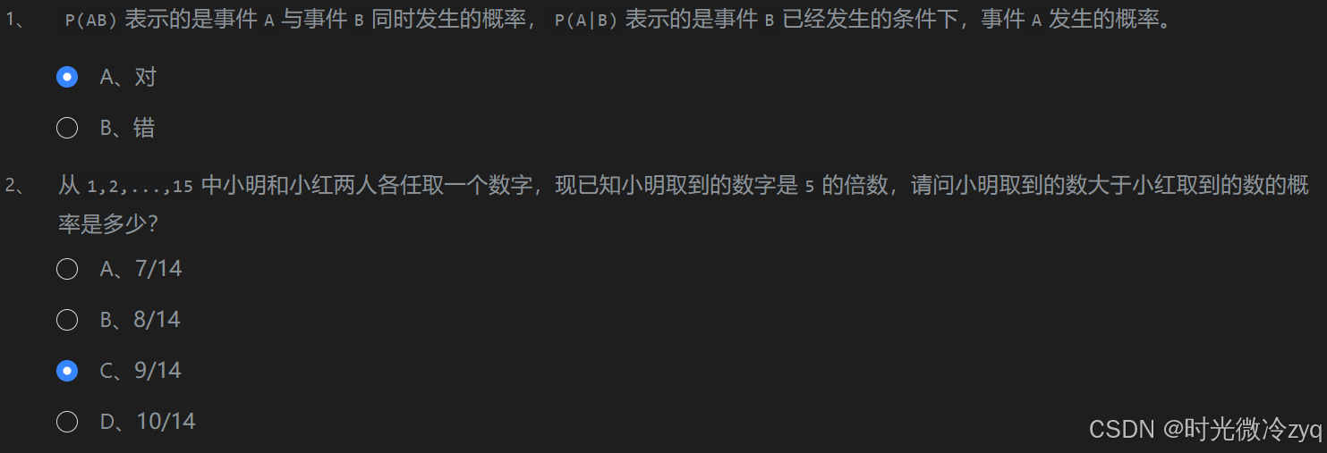
1、条件概率
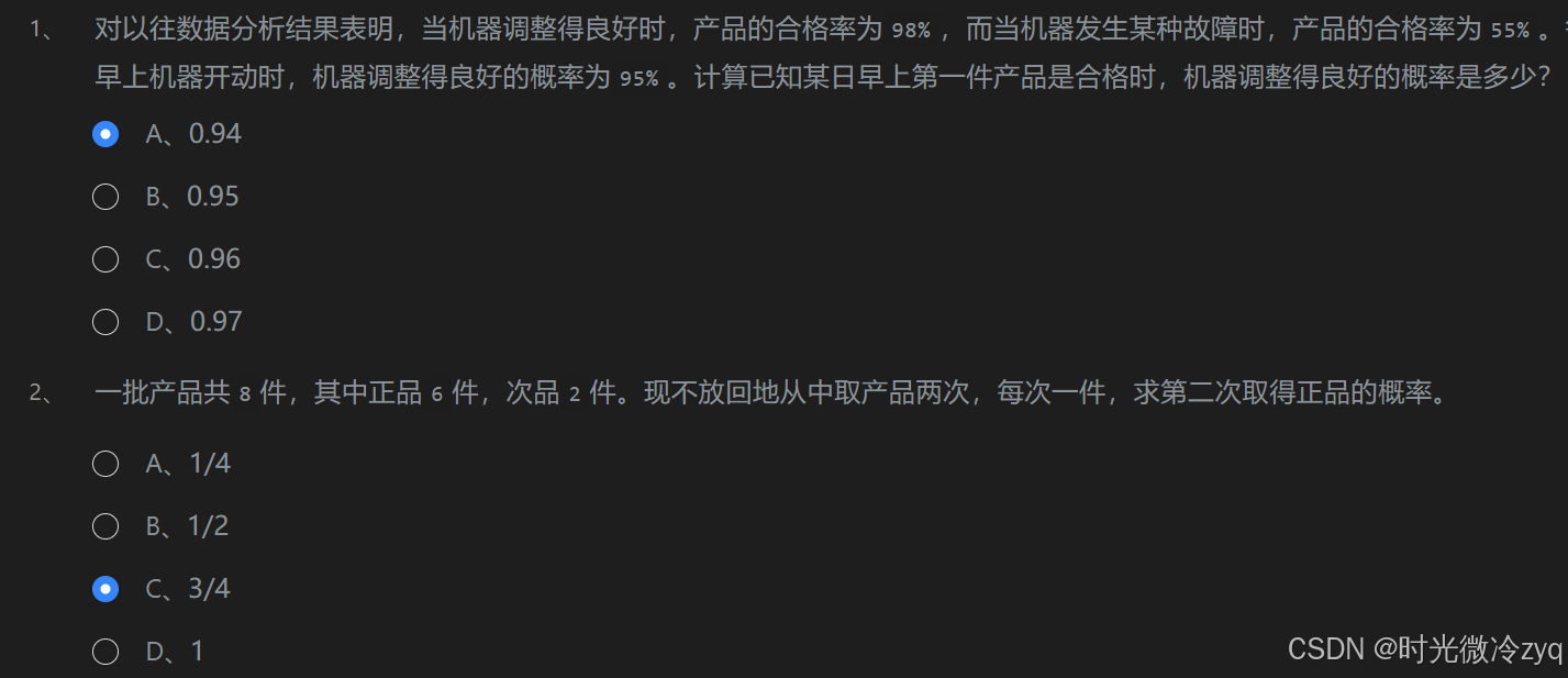
2、贝叶斯公式
3、朴素贝叶斯分类算法流程
import numpy as np

class NaiveBayesClassifier(object):
    def __init__(self):
        self.label_prob = {}
        self.condition_prob = {}

    def fit(self, feature, label):
        # 计算标签的概率
        unique_labels, counts = np.unique(label, return_counts=True)
        total_samples = len(label)
        for label, count in zip(unique_labels, counts):
            self.label_prob[label] = (count + 1) / (total_samples + len(unique_labels))  # Laplace smoothing

        # 计算条件概率
        for label in unique_labels:
            self.condition_prob[label] = {}
            # 只考虑当前标签的数据
            subset = feature[label == label]
            for i in range(feature.shape[1]):
                unique_features, counts = np.unique(subset[:, i], return_counts=True)
                total_feature_count = len(subset)
                self.condition_prob[label][i] = {feat: (cnt + 1) / (total_feature_count + len(unique_features))
                                                 for feat, cnt in zip(unique_features, counts)}

    def predict(self, feature):
        predictions = []
        for sample in feature:
            max_posterior = -np.inf
            predicted_label = None
            for label in self.label_prob.keys():
                posterior = np.log(self.label_prob[label])
                for i, value in enumerate(sample):
                    if value in self.condition_prob[label][i]:
                        posterior += np.log(self.condition_prob[label][i][value])
                if posterior > max_posterior:
                    max_posterior = posterior
                    predicted_label = label
            predictions.append(predicted_label)
        return np.array(predictions)

# 使用示例
X = np.array([[2, 1, 1],
              [1, 2, 2],
              [2, 2, 2],
              [2, 1, 2],
              [1, 2, 3],
              [2, 1, 1]])
y = np.array([1, 0, 1, 0, 1, 0])

nb_classifier = NaiveBayesClassifier()
nb_classifier.fit(X, y)

# 假设我们有一个新的样本需要预测
new_sample = np.array([[1, 2, 2]])
prediction = nb_classifier.predict(new_sample)
#print("预测结果:", prediction)4、拉普拉斯平滑
import numpy as np

class NaiveBayesClassifier(object):
    def __init__(self):
        self.label_prob = {}
        self.condition_prob = {}

    def fit(self, feature, label):
        # 计算标签的先验概率
        unique_labels, counts = np.unique(label, return_counts=True)
        total_samples = len(label)
        for label, count in zip(unique_labels, counts):
            self.label_prob[label] = (count + 1) / (total_samples + len(unique_labels))  # 拉普拉斯平滑

        # 初始化条件概率字典
        self.condition_prob = {label: {} for label in unique_labels}

        # 对于每个特征列
        for i in range(feature.shape[1]):
            # 获取当前特征的所有可能取值
            unique_features = np.unique(feature[:, i])
            # 对于每个类别
            for label in unique_labels:
                # 只考虑当前类别的数据
                subset = feature[label == label]
                # 初始化当前特征的条件概率
                self.condition_prob[label][i] = {feat: 1 / (len(subset) + len(unique_features)) for feat in unique_features}
                # 更新条件概率
                for feat in unique_features:
                    self.condition_prob[label][i][feat] = (np.sum(subset[:, i] == feat) + 1) / (len(subset) + len(unique_features))

    def predict(self, feature):
        result = []
        # 对每条测试数据都进行预测
        for f in feature:
            # 可能的类别的概率
            prob = np.zeros(len(self.label_prob.keys()))
            ii = 0
            for label, label_prob in self.label_prob.items():
                # 计算概率
                prob[ii] = label_prob
                for j in range(len(f)):
                    if f[j] in self.condition_prob[label][j]:
                        prob[ii] *= self.condition_prob[label][j][f[j]]
                    else:
                        prob[ii] *= 1e-10  # 如果特征值未出现在训练集中,则赋予一个很小的概率
                ii += 1
            # 取概率最大的类别作为结果
            result.append(list(self.label_prob.keys())[np.argmax(prob)])
        return np.array(result)

# 使用示例
X = np.array([[2, 1, 1],
              [1, 2, 2],
              [2, 2, 2],
              [2, 1, 2],
              [1, 2, 3],
              [2, 1, 2]])
y = np.array([1, 0, 1, 1, 1, 0])

nb_classifier = NaiveBayesClassifier()
nb_classifier.fit(X, y)

# 假设我们有一个新的样本需要预测
new_sample = np.array([[1, 2, 2]])
prediction = nb_classifier.predict(new_sample)
#print("预测结果:", prediction)5、新闻文本主题分类
from sklearn.feature_extraction.text import CountVectorizer  # 从sklearn.feature_extraction.text里导入文本特征向量化模块
from sklearn.naive_bayes import MultinomialNB
from sklearn.feature_extraction.text import TfidfTransformer
def news_predict(train_sample, train_label, test_sample):
    '''
    训练模型并进行预测,返回预测结果
    :param train_sample:原始训练集中的新闻文本,类型为ndarray
    :param train_label:训练集中新闻文本对应的主题标签,类型为ndarray
    :test_sample:原始测试集中的新闻文本,类型为ndarray
    '''
    # ********* Begin *********#
    vec = CountVectorizer()
    train_sample = vec.fit_transform(train_sample)
    test_sample = vec.transform(test_sample)
    tfidf = TfidfTransformer()
    train_sample = tfidf.fit_transform(train_sample)
    test_sample = tfidf.transform(test_sample)
    mnb = MultinomialNB(alpha=0.01)  # 使用默认配置初始化朴素贝叶斯
    mnb.fit(train_sample, train_label)  # 利用训练数据对模型参数进行估计
    predict = mnb.predict(test_sample)  # 对参数进行预测
    return predict
    # ********* End *********#
4、感知机
1、感知机 - 西瓜好坏自动识别
#encoding=utf8
import numpy as np
#构建感知机算法
class Perceptron(object):
    def __init__(self, learning_rate = 0.01, max_iter = 200):
        self.lr = learning_rate
        self.max_iter = max_iter
    def fit(self, data, label):
        '''
        input:data(ndarray):训练数据特征
              label(ndarray):训练数据标签
        output:w(ndarray):训练好的权重
               b(ndarry):训练好的偏置
        '''
        #编写感知机训练方法,w为权重,b为偏置
        self.w = np.array([1.]*data.shape[1])
        self.b = np.array([1.])
        #********* Begin *********#
        i = 0
        while i < self.max_iter:
            flag = True
            for j in range(len(label)):
                if label[j] * (np.inner(self.w, data[j]) + self.b) <= 0:
                    flag = False
                    self.w += self.lr * (label[j] * data[j])
                    self.b += self.lr * label[j]
            if flag:
                break
            i+=1
        #********* End *********#
    def predict(self, data):
        '''
        input:data(ndarray):测试数据特征
        output:predict(ndarray):预测标签
        '''
        #********* Begin *********#
        y = np.inner(data, self.w) + self.b
        for i in range(len(y)): # range(0,6)
            if y[i] >= 0:
                y[i] = 1
            else:
                y[i] = -1
        predict = y

        #********* End *********#
        return predict
2、scikit-learn感知机实践 - 癌细胞精准识别
#encoding=utf8
import os

if os.path.exists('./step2/result.csv'):
    os.remove('./step2/result.csv')

#********* Begin *********#
import pandas as pd
train_data = pd.read_csv('./step2/train_data.csv')
train_label = pd.read_csv('./step2/train_label.csv')
train_label = train_label['target']
test_data = pd.read_csv('./step2/test_data.csv')
from sklearn.linear_model.perceptron import Perceptron
clf = Perceptron(eta0 = 0.01,max_iter = 200)
clf.fit(train_data, train_label)
result = clf.predict(test_data)
frameResult = pd.DataFrame({'result':result})
frameResult.to_csv('./step2/result.csv', index = False)
#********* End *********#
5、EM算法
1、极大似然估计

2、实现EM算法的单次迭代过程
import numpy as np
from scipy import stats

def em_single(init_values, observations):
    """
    模拟抛掷硬币实验并估计在一次迭代中,硬币A与硬币B正面朝上的概率
    :param init_values:硬币A与硬币B正面朝上的概率的初始值,类型为list,如[0.2, 0.7]代表硬币A正面朝上的概率为0.2,硬币B正面朝上的概率为0.7。
    :param observations:抛掷硬币的实验结果记录,类型为list。
    :return:将估计出来的硬币A和硬币B正面朝上的概率组成list返回。如[0.4, 0.6]表示你认为硬币A正面朝上的概率为0.4,硬币B正面朝上的概率为0.6。
    """
    #********* Begin *********#
    observations = np.array(observations)
    counts = {'A': {'H': 0, 'T': 0}, 'B': {'H': 0, 'T': 0}}
    theta_A = init_values[0]
    theta_B = init_values[1]
    # E step
    for observation in observations:
        len_observation = len(observation)
        num_heads = observation.sum()
        num_tails = len_observation - num_heads
        # 两个二项分布
        contribution_A = stats.binom.pmf(num_heads, len_observation, theta_A)
        contribution_B = stats.binom.pmf(num_heads, len_observation, theta_B)
        weight_A = contribution_A / (contribution_A + contribution_B)
        weight_B = contribution_B / (contribution_A + contribution_B)
        # 更新在当前参数下A、B硬币产生的正反面次数
        counts['A']['H'] += weight_A * num_heads
        counts['A']['T'] += weight_A * num_tails
        counts['B']['H'] += weight_B * num_heads
        counts['B']['T'] += weight_B * num_tails
    # M step
    new_theta_A = counts['A']['H'] / (counts['A']['H'] + counts['A']['T'])
    new_theta_B = counts['B']['H'] / (counts['B']['H'] + counts['B']['T'])
    return [new_theta_A, new_theta_B]

    #********* End *********#
3、实现EM算法的主循环
import numpy as np
from scipy import stats


def em_single(init_values, observations):
    """
    模拟抛掷硬币实验并估计在一次迭代中,硬币A与硬币B正面朝上的概率。请不要修改!!
    :param init_values:硬币A与硬币B正面朝上的概率的初始值,类型为list,如[0.2, 0.7]代表硬币A正面朝上的概率为0.2,硬币B正面朝上的概率为0.7。
    :param observations:抛掷硬币的实验结果记录,类型为list。
    :return:将估计出来的硬币A和硬币B正面朝上的概率组成list返回。如[0.4, 0.6]表示你认为硬币A正面朝上的概率为0.4,硬币B正面朝上的概率为0.6。
    """
    observations = np.array(observations)
    counts = {'A': {'H': 0, 'T': 0}, 'B': {'H': 0, 'T': 0}}
    theta_A = init_values[0]
    theta_B = init_values[1]
    # E step
    for observation in observations:
        len_observation = len(observation)
        num_heads = observation.sum()
        num_tails = len_observation - num_heads
        # 两个二项分布
        contribution_A = stats.binom.pmf(num_heads, len_observation, theta_A)
        contribution_B = stats.binom.pmf(num_heads, len_observation, theta_B)
        weight_A = contribution_A / (contribution_A + contribution_B)
        weight_B = contribution_B / (contribution_A + contribution_B)
        # 更新在当前参数下A、B硬币产生的正反面次数
        counts['A']['H'] += weight_A * num_heads
        counts['A']['T'] += weight_A * num_tails
        counts['B']['H'] += weight_B * num_heads
        counts['B']['T'] += weight_B * num_tails
    # M step
    new_theta_A = counts['A']['H'] / (counts['A']['H'] + counts['A']['T'])
    new_theta_B = counts['B']['H'] / (counts['B']['H'] + counts['B']['T'])
    return [new_theta_A, new_theta_B]

def em(observations, thetas, tol=1e-4, iterations=100):
    """
    模拟抛掷硬币实验并使用EM算法估计硬币A与硬币B正面朝上的概率。
    :param observations: 抛掷硬币的实验结果记录,类型为list。
    :param thetas: 硬币A与硬币B正面朝上的概率的初始值,类型为list,如[0.2, 0.7]代表硬币A正面朝上的概率为0.2,硬币B正面朝上的概率为0.7。
    :param tol: 差异容忍度,即当EM算法估计出来的参数theta不怎么变化时,可以提前挑出循环。例如容忍度为1e-4,则表示若这次迭代的估计结果与上一次迭代的估计结果之间的L1距离小于1e-4则跳出循环。为了正确的评测,请不要修改该值。
    :param iterations: EM算法的最大迭代次数。为了正确的评测,请不要修改该值。
    :return: 将估计出来的硬币A和硬币B正面朝上的概率组成list或者ndarray返回。如[0.4, 0.6]表示你认为硬币A正面朝上的概率为0.4,硬币B正面朝上的概率为0.6。
    """
    #********* Begin *********#
    theta = np.array(thetas)#初始值
    # 循环iterations次
    for i in range(iterations):
        new_theta = np.array(em_single(theta, observations))
    # 当差异小于iterations跳出循环
        if np.sum(np.abs(new_theta-theta))<tol:
            break;
        theta = new_theta
    return theta
    #********* End *********#
6、神经网络
1、神经网络基本概念

2、激活函数
#encoding=utf8

def relu(x):
    '''
    x:负无穷到正无穷的实数
    '''
    #********* Begin *********#
    if x<=0:
        return 0
    else:
        return x
    #********* End *********#
3、反向传播算法
#encoding=utf8
import os
import pandas as pd
from sklearn.neural_network import MLPClassifier
if os.path.exists('./step2/result.csv'):
    os.remove('./step2/result.csv')

#********* Begin *********#
train_data = pd.read_csv('./step2/train_data.csv')
train_label = pd.read_csv('./step2/train_label.csv')
train_label = train_label['target']
test_data = pd.read_csv('./step2/test_data.csv')
mlp = MLPClassifier(solver='lbfgs',max_iter=30, alpha=1e-4,hidden_layer_sizes=(20, ))
mlp.fit(train_data, train_label)
predict = mlp.predict(test_data)
df = pd.DataFrame({'result':predict})
df.to_csv('./step2/result.csv', index=False)
#********* End *********#
4、使用pytorch搭建卷积神经网络识别手写数字
#encoding=utf8
import torch
import torch.nn as nn
from torch.autograd import Variable
import torch.utils.data as Data
import torchvision
import os
if os.path.exists('./step3/cnn.pkl'):
    os.remove('./step3/cnn.pkl')

#加载数据
train_data = torchvision.datasets.MNIST(
    root='./step3/mnist/',
    train=True,                                     # this is training data
    transform=torchvision.transforms.ToTensor(),    # Converts a PIL.Image or numpy.ndarray to
    download=False,
)
#取6000个样本为训练集
train_data_tiny = []

for i in range(6000):
    train_data_tiny.append(train_data[i])

train_data = train_data_tiny

#********* Begin *********#
train_loader = Data.DataLoader(
    dataset=train_data,
    batch_size=64,
    num_workers=2,
    shuffle=True
)
# 构建卷积神经网络模型
class CNN(nn.Module):
    def __init__(self):
        super(CNN, self).__init__()
        self.conv1 = nn.Sequential(  # input shape (1, 28, 28)
            nn.Conv2d(
                in_channels=1,  # input height
                out_channels=16,  # n_filters
                kernel_size=5,  # filter size
                stride=1,  # filter movement/step
                padding=2,
                # if want same width and length of this image after con2d, padding=(kernel_size-1)/2 if stride=1
            ),  # output shape (16, 28, 28)
            nn.ReLU(),  # activation
            nn.MaxPool2d(kernel_size=2),  # choose max value in 2x2 area, output shape (16, 14, 14)
        )
        self.conv2 = nn.Sequential(  # input shape (16, 14, 14)
            nn.Conv2d(16, 32, 5, 1, 2),  # output shape (32, 14, 14)
            nn.ReLU(),  # activation
            nn.MaxPool2d(2),  # output shape (32, 7, 7)
        )
        self.out = nn.Linear(32 * 7 * 7, 10)  # fully connected layer, output 10 classes
    def forward(self, x):
        x = self.conv1(x)
        x = self.conv2(x)
        x = x.view(x.size(0), -1)  # flatten the output of conv2 to (batch_size, 32 * 7 * 7)
        output = self.out(x)
        return output
cnn = CNN()
# SGD表示使用随机梯度下降方法,lr为学习率,momentum为动量项系数
optimizer = torch.optim.SGD(cnn.parameters(), lr=0.01, momentum=0.9)
# 交叉熵损失函数
loss_func = nn.CrossEntropyLoss()
EPOCH = 3
for e in range(EPOCH):
    for x, y in train_loader:
        batch_x = Variable(x)
        batch_y = Variable(y)
        outputs = cnn(batch_x)
        loss = loss_func(outputs, batch_y)
        optimizer.zero_grad()
        loss.backward()
        optimizer.step()

#********* End *********#
#保存模型
torch.save(cnn.state_dict(), './step3/cnn.pkl')
7、支持向量回归
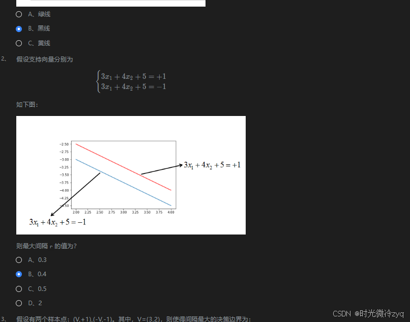
1、线性可分支持向量机
2、线性支持向量机
#encoding=utf8
from sklearn.svm import LinearSVC

def linearsvc_predict(train_data,train_label,test_data):
    '''
    input:train_data(ndarray):训练数据
          train_label(ndarray):训练标签
    output:predict(ndarray):测试集预测标签
    '''
    #********* Begin *********#
    clf = LinearSVC(dual=False)
    clf.fit(train_data,train_label)
    predict = clf.predict(test_data)
    #********* End *********#
    return predict
3、非线性支持向量机
#encoding=utf8
from sklearn.svm import SVC

def svc_predict(train_data,train_label,test_data,kernel):
    '''
    input:train_data(ndarray):训练数据
          train_label(ndarray):训练标签
          kernel(str):使用核函数类型:
              'linear':线性核函数
              'poly':多项式核函数
              'rbf':径像核函数/高斯核
    output:predict(ndarray):测试集预测标签
    '''
    #********* Begin *********#
    clf =SVC(kernel=kernel)
    clf.fit(train_data,train_label)
    predict = clf.predict(test_data)
    #********* End *********#
    return predict
4、序列最小优化算法
#encoding=utf8
import numpy as np
class smo:
    def __init__(self, max_iter=100, kernel='linear'):
        '''
        input:max_iter(int):最大训练轮数
              kernel(str):核函数,等于'linear'表示线性,等于'poly'表示多项式
        '''
        self.max_iter = max_iter
        self._kernel = kernel
    #初始化模型
    def init_args(self, features, labels):
        self.m, self.n = features.shape
        self.X = features
        self.Y = labels
        self.b = 0.0
        # 将Ei保存在一个列表里
        self.alpha = np.ones(self.m)
        self.E = [self._E(i) for i in range(self.m)]
        # 错误惩罚参数
        self.C = 1.0
    #********* Begin *********#
    #kkt条件
    def _KKT(self, i):
        y_g = self._g(i)*self.Y[i]
        if self.alpha[i] == 0:
            return y_g >= 1
        elif 0 < self.alpha[i] < self.C:
            return y_g == 1
        else:
            return y_g <= 1
    # g(x)预测值,输入xi(X[i])
    def _g(self, i):
        r = self.b
        for j in range(self.m):
            r += self.alpha[j]*self.Y[j]*self.kernel(self.X[i], self.X[j])
        return r
    # 核函数,多项式添加二次项即可
    def kernel(self, x1, x2):
        if self._kernel == 'linear':
            return sum([x1[k]*x2[k] for k in range(self.n)])
        elif self._kernel == 'poly':
            return (sum([x1[k]*x2[k] for k in range(self.n)]) + 1)**2
        return 0
    # E(x)为g(x)对输入x的预测值和y的差
    def _E(self, i):
        return self._g(i) - self.Y[i]
    #初始alpha
    def _init_alpha(self):
        # 外层循环首先遍历所有满足0<a<C的样本点,检验是否满足KKT
        index_list = [i for i in range(self.m) if 0 < self.alpha[i] < self.C]
        # 否则遍历整个训练集
        non_satisfy_list = [i for i in range(self.m) if i not in index_list]
        index_list.extend(non_satisfy_list)
        for i in index_list:
            if self._KKT(i):
                continue
            E1 = self.E[i]
            # 如果E2是+,选择最小的;如果E2是负的,选择最大的
            if E1 >= 0:
                j = min(range(self.m), key=lambda x: self.E[x])
            else:
                j = max(range(self.m), key=lambda x: self.E[x])
            return i, j
    #选择alpha参数
    def _compare(self, _alpha, L, H):
        if _alpha > H:
            return H
        elif _alpha < L:
            return L
        else:
            return _alpha
    #训练
    def fit(self, features, labels):
        '''
        input:features(ndarray):特征
              label(ndarray):标签
        '''
        self.init_args(features, labels)
        for t in range(self.max_iter):
            i1, i2 = self._init_alpha()
            # 边界
            if self.Y[i1] == self.Y[i2]:
                L = max(0, self.alpha[i1]+self.alpha[i2]-self.C)
                H = min(self.C, self.alpha[i1]+self.alpha[i2])
            else:
                L = max(0, self.alpha[i2]-self.alpha[i1])
                H = min(self.C, self.C+self.alpha[i2]-self.alpha[i1])
            E1 = self.E[i1]
            E2 = self.E[i2]
            # eta=K11+K22-2K12
            eta = self.kernel(self.X[i1], self.X[i1]) + self.kernel(self.X[i2], self.X[i2]) - 2*self.kernel(self.X[i1], self.X[i2])
            if eta <= 0:
                continue
            alpha2_new_unc = self.alpha[i2] + self.Y[i2] * (E2 - E1) / eta
            alpha2_new = self._compare(alpha2_new_unc, L, H)
            alpha1_new = self.alpha[i1] + self.Y[i1] * self.Y[i2] * (self.alpha[i2] - alpha2_new)
            b1_new = -E1 - self.Y[i1] * self.kernel(self.X[i1], self.X[i1]) * (alpha1_new-self.alpha[i1]) - self.Y[i2] * self.kernel(self.X[i2], self.X[i1]) * (alpha2_new-self.alpha[i2])+ self.b
            b2_new = -E2 - self.Y[i1] * self.kernel(self.X[i1], self.X[i2]) * (alpha1_new-self.alpha[i1]) - self.Y[i2] * self.kernel(self.X[i2], self.X[i2]) * (alpha2_new-self.alpha[i2])+ self.b
            if 0 < alpha1_new < self.C:
                b_new = b1_new
            elif 0 < alpha2_new < self.C:
                b_new = b2_new
            else:
                # 选择中点
                b_new = (b1_new + b2_new) / 2
            # 更新参数
            self.alpha[i1] = alpha1_new
            self.alpha[i2] = alpha2_new
            self.b = b_new
            self.E[i1] = self._E(i1)
            self.E[i2] = self._E(i2)
    def predict(self, data):
        '''
        input:data(ndarray):单个样本
        output:预测为正样本返回+1,负样本返回-1
        '''
        r = self.b
        for i in range(self.m):
            r += self.alpha[i] * self.Y[i] * self.kernel(data, self.X[i])
        return 1 if r > 0 else -1
    #********* End *********#
5、支持向量回归
#encoding=utf8
from sklearn.svm import SVR

def svr_predict(train_data,train_label,test_data):
    '''
    input:train_data(ndarray):训练数据
          train_label(ndarray):训练标签
    output:predict(ndarray):测试集预测标签
    '''
    #********* Begin *********#
    svr = SVR(kernel='rbf',C=100,gamma= 0.001,epsilon=0.1)
    svr.fit(train_data,train_label)
    predict = svr.predict(test_data)

    #********* End *********#
    return predict
8、模型评估、选择与验证
1、为什么要有训练集与测试集

2、欠拟合与过拟合

3、偏差与方差

4、验证集与交叉验证
5、衡量回归的性能指标
6、准确度的陷阱与混淆矩阵
import numpy as np

def confusion_matrix(y_true, y_predict):
    '''
    构建二分类的混淆矩阵,并将其返回
    :param y_true: 真实类别,类型为ndarray
    :param y_predict: 预测类别,类型为ndarray
    :return: shape为(2, 2)的ndarray
    '''

    #********* Begin *********#
    def TN(y_true,y_predict):
        return np.sum((y_true==0) &  (y_predict==0))
    def FP(y_true,y_predict):
        return np.sum((y_true==0) & (y_predict==1))
    def FN (y_true,y_predict):
        return np.sum((y_true==1)&   (y_predict==0))
    def TP(y_true,y_predict):
        return np.sum((y_true==1)&  (y_predict==1))
    return np.array([
        [TN(y_true,y_predict),FP(y_true,y_predict)],
        [FN(y_true,y_predict),TP(y_true,y_predict)]
    ])
    #********* End *********#
7、精准率与召回率
import numpy as np

def precision_score(y_true, y_predict):
    '''
    计算精准率并返回
    :param y_true: 真实类别,类型为ndarray
    :param y_predict: 预测类别,类型为ndarray
    :return: 精准率,类型为float
    '''

    #********* Begin *********#
    def TN(y_true,y_predict):
        return np.sum((y_true==0) & (y_predict==0))
    def FP(y_true,y_predict):
        return np.sum((y_true==0)& (y_predict==1))
    def FN(y_true,y_predict):
        return np.sum((y_true==1) & (y_predict==0))
    def TP(y_true,y_predict):
        return np.sum((y_true==1)&  (y_predict==1))
    return TP(y_true,y_predict)/(TP(y_true,y_predict)+FP(y_true,y_predict))
    #********* End *********#


def recall_score(y_true, y_predict):
    '''
    计算召回率并召回
    :param y_true: 真实类别,类型为ndarray
    :param y_predict: 预测类别,类型为ndarray
    :return: 召回率,类型为float
    '''

    #********* Begin *********#
    def TP(y_true,y_predict):
        return np.sum((y_true==1) & (y_predict==1))
    def FN(y_true,y_predict):
        return np.sum((y_true==1)& (y_predict==0))
    tp=TP(y_true,y_predict)
    fn=FN(y_true,y_predict)
    try:
        return tp/(tp+fn)
    except:
        return 0.0
    #********* End *********#
8、F1 Score
import numpy as np

def f1_score(precision, recall):
    '''
    计算f1 score并返回
    :param precision: 模型的精准率,类型为float
    :param recall: 模型的召回率,类型为float
    :return: 模型的f1 score,类型为float
    '''
    #********* Begin *********#
    score=(2*precision*recall)/(precision+recall)
    return score
    #********* End ***********#
9、ROC曲线与AUC
import numpy as np

def calAUC(prob, labels):
    '''
    计算AUC并返回
    :param prob: 模型预测样本为Positive的概率列表,类型为ndarray
    :param labels: 样本的真实类别列表,其中1表示Positive,0表示Negtive,类型为ndarray
    :return: AUC,类型为float
    '''

    #********* Begin *********#
    f=list(zip(prob,labels))
    rank=[values2 for values1,values2 in sorted(f,key=lambda x:x[0])]
    rankList=[i+1 for  i in range(len(rank)) if rank[i]==1]
    posNum=0
    negNum=0
    for i in range(len(labels)):
        if(labels[i]==1):
            posNum+=1
        else:
            negNum+=1
    auc=(sum(rankList)-(posNum*(posNum+1))/2)/(posNum*negNum)
    return auc
    #********* End *********#
10、sklearn中的分类性能指标
from sklearn.metrics import accuracy_score, precision_score, recall_score, f1_score, roc_auc_score

def classification_performance(y_true, y_pred, y_prob):
    '''
    返回准确度、精准率、召回率、f1 Score和AUC
    :param y_true:样本的真实类别,类型为`ndarray`
    :param y_pred:模型预测出的类别,类型为`ndarray`
    :param y_prob:模型预测样本为`Positive`的概率,类型为`ndarray`
    :return:
    '''

    #********* Begin *********#
    a=accuracy_score(y_true,y_pred)
    b=precision_score(y_true,y_pred)
    c=recall_score(y_true,y_pred)
    d=f1_score(y_true,y_pred)
    e=roc_auc_score(y_true,y_prob)
    return (a,b,c,d,e)
    #********* End *********#
仅供机器学习参考使用!

魔乐社区(Modelers.cn) 是一个中立、公益的人工智能社区,提供人工智能工具、模型、数据的托管、展示与应用协同服务,为人工智能开发及爱好者搭建开放的学习交流平台。社区通过理事会方式运作,由全产业链共同建设、共同运营、共同享有,推动国产AI生态繁荣发展。
更多推荐


 11
11 0
0- 0


 已为社区贡献2条内容

所有评论(0)