Python基础(十三) 机器学习sklearn库详解与应用_e anad lib site-packages sklearn linear_model _lo(1)
| 123 | 4.9 | 1.8 | 2 |
| 124 | 5.7 | 2.1 | 2 |
| 125 | 6.0 | 1.8 | 2 |
| 126 | 4.8 | 1.8 | 2 |
| 127 | 4.9 | 1.8 | 2 |
| 128 | 5.6 | 2.1 | 2 |
| 129 | 5.8 | 1.6 | 2 |
| 130 | 6.1 | 1.9 | 2 |
| 131 | 6.4 | 2.0 | 2 |
| 132 | 5.6 | 2.2 | 2 |
| 133 | 5.1 | 1.5 | 2 |
| 134 | 5.6 | 1.4 | 2 |
| 135 | 6.1 | 2.3 | 2 |
| 136 | 5.6 | 2.4 | 2 |
| 137 | 5.5 | 1.8 | 2 |
| 138 | 4.8 | 1.8 | 2 |
| 139 | 5.4 | 2.1 | 2 |
| 140 | 5.6 | 2.4 | 2 |
| 141 | 5.1 | 2.3 | 2 |
| 142 | 5.1 | 1.9 | 2 |
| 143 | 5.9 | 2.3 | 2 |
| 144 | 5.7 | 2.5 | 2 |
| 145 | 5.2 | 2.3 | 2 |
| 146 | 5.0 | 1.9 | 2 |
| 147 | 5.2 | 2.0 | 2 |
| 148 | 5.4 | 2.3 | 2 |
| 149 | 5.1 | 1.8 | 2 |
150 rows × 3 columns
【5】数据集的标准化(本数据集特征比较接近,实际处理过程中未标准化)
from sklearn.preprocessing import StandardScaler
import pandas as pd
trans = StandardScaler()
_iris_simple = trans.fit_transform(iris_simple[["petal\_length", "petal\_width"]])
_iris_simple = pd.DataFrame(_iris_simple, columns = ["petal\_length", "petal\_width"])
_iris_simple.describe()
| petal_length | petal_width | |
|---|---|---|
| count | 1.500000e+02 | 1.500000e+02 |
| mean | -8.652338e-16 | -4.662937e-16 |
| std | 1.003350e+00 | 1.003350e+00 |
| min | -1.567576e+00 | -1.447076e+00 |
| 25% | -1.226552e+00 | -1.183812e+00 |
| 50% | 3.364776e-01 | 1.325097e-01 |
| 75% | 7.627583e-01 | 7.906707e-01 |
| max | 1.785832e+00 | 1.712096e+00 |
【6】构建训练集和测试集(本课暂不考虑验证集)
from sklearn.model_selection import train_test_split

train_set, test_set = train_test_split(iris_simple, test_size=0.2) # 20%的数据作为测试集
test_set.head()
| petal_length | petal_width | species | |
|---|---|---|---|
| 3 | 1.5 | 0.2 | 0 |
| 111 | 5.3 | 1.9 | 2 |
| 24 | 1.9 | 0.2 | 0 |
| 5 | 1.7 | 0.4 | 0 |
| 92 | 4.0 | 1.2 | 1 |
iris_x_train = train_set[["petal\_length", "petal\_width"]]
iris_x_train.head()
| petal_length | petal_width | |
|---|---|---|
| 63 | 4.7 | 1.4 |
| 93 | 3.3 | 1.0 |
| 34 | 1.5 | 0.2 |
| 35 | 1.2 | 0.2 |
| 126 | 4.8 | 1.8 |
iris_y_train = train_set["species"].copy()
iris_y_train.head()
63     1
93     1
34     0
35     0
126    2
Name: species, dtype: int32
iris_x_test = test_set[["petal\_length", "petal\_width"]]
iris_x_test.head()
| petal_length | petal_width | |
|---|---|---|
| 3 | 1.5 | 0.2 |
| 111 | 5.3 | 1.9 |
| 24 | 1.9 | 0.2 |
| 5 | 1.7 | 0.4 |
| 92 | 4.0 | 1.2 |
iris_y_test = test_set["species"].copy()
iris_y_test.head()
3      0
111    2
24     0
5      0
92     1
Name: species, dtype: int32
13.1 k近邻算法
【1】基本思想
与待预测点最近的训练数据集中的k个邻居
把k个近邻中最常见的类别预测为带预测点的类别
【2】sklearn实现
from sklearn.neighbors import KNeighborsClassifier
- 构建分类器对象
clf = KNeighborsClassifier()
clf
KNeighborsClassifier(algorithm='auto', leaf_size=30, metric='minkowski',
                     metric_params=None, n_jobs=None, n_neighbors=5, p=2,
                     weights='uniform')
- 训练
clf.fit(iris_x_train, iris_y_train)
KNeighborsClassifier(algorithm='auto', leaf_size=30, metric='minkowski',
                     metric_params=None, n_jobs=None, n_neighbors=5, p=2,
                     weights='uniform')
- 预测
res = clf.predict(iris_x_test)
print(res)
print(iris_y_test.values)
[0 2 0 0 1 1 0 2 1 2 1 2 2 2 1 0 0 0 1 0 2 0 2 1 0 1 0 0 1 1]
[0 2 0 0 1 1 0 2 2 2 1 2 2 2 1 0 0 0 1 0 2 0 2 1 0 1 0 0 1 1]
- 翻转
encoder.inverse_transform(res)
array(['setosa', 'virginica', 'setosa', 'setosa', 'versicolor',
       'versicolor', 'setosa', 'virginica', 'versicolor', 'virginica',
       'versicolor', 'virginica', 'virginica', 'virginica', 'versicolor',
       'setosa', 'setosa', 'setosa', 'versicolor', 'setosa', 'virginica',
       'setosa', 'virginica', 'versicolor', 'setosa', 'versicolor',
       'setosa', 'setosa', 'versicolor', 'versicolor'], dtype=object)
- 评估
accuracy = clf.score(iris_x_test, iris_y_test)
print("预测正确率:{:.0%}".format(accuracy))
预测正确率:97%
- 存储数据
out = iris_x_test.copy()
out["y"] = iris_y_test
out["pre"] = res
out
| petal_length | petal_width | y | pre | |
|---|---|---|---|---|
| 3 | 1.5 | 0.2 | 0 | 0 |
| 111 | 5.3 | 1.9 | 2 | 2 |
| 24 | 1.9 | 0.2 | 0 | 0 |
| 5 | 1.7 | 0.4 | 0 | 0 |
| 92 | 4.0 | 1.2 | 1 | 1 |
| 57 | 3.3 | 1.0 | 1 | 1 |
| 1 | 1.4 | 0.2 | 0 | 0 |
| 112 | 5.5 | 2.1 | 2 | 2 |
| 106 | 4.5 | 1.7 | 2 | 1 |
| 136 | 5.6 | 2.4 | 2 | 2 |
| 80 | 3.8 | 1.1 | 1 | 1 |
| 131 | 6.4 | 2.0 | 2 | 2 |
| 147 | 5.2 | 2.0 | 2 | 2 |
| 113 | 5.0 | 2.0 | 2 | 2 |
| 84 | 4.5 | 1.5 | 1 | 1 |
| 39 | 1.5 | 0.2 | 0 | 0 |
| 40 | 1.3 | 0.3 | 0 | 0 |
| 17 | 1.4 | 0.3 | 0 | 0 |
| 56 | 4.7 | 1.6 | 1 | 1 |
| 2 | 1.3 | 0.2 | 0 | 0 |
| 100 | 6.0 | 2.5 | 2 | 2 |
| 42 | 1.3 | 0.2 | 0 | 0 |
| 144 | 5.7 | 2.5 | 2 | 2 |
| 79 | 3.5 | 1.0 | 1 | 1 |
| 19 | 1.5 | 0.3 | 0 | 0 |
| 75 | 4.4 | 1.4 | 1 | 1 |
| 44 | 1.9 | 0.4 | 0 | 0 |
| 37 | 1.4 | 0.1 | 0 | 0 |
| 64 | 3.6 | 1.3 | 1 | 1 |
| 90 | 4.4 | 1.2 | 1 | 1 |
out.to_csv("iris\_predict.csv")
【3】可视化
import numpy as np
import matplotlib as mpl
import matplotlib.pyplot as plt

def draw(clf):

    # 网格化
    M, N = 500, 500
    x1_min, x2_min = iris_simple[["petal\_length", "petal\_width"]].min(axis=0)
    x1_max, x2_max = iris_simple[["petal\_length", "petal\_width"]].max(axis=0)
    t1 = np.linspace(x1_min, x1_max, M)
    t2 = np.linspace(x2_min, x2_max, N)
    x1, x2 = np.meshgrid(t1, t2)

    # 预测
    x_show = np.stack((x1.flat, x2.flat), axis=1)
    y_predict = clf.predict(x_show)

    # 配色
    cm_light = mpl.colors.ListedColormap(["#A0FFA0", "#FFA0A0", "#A0A0FF"])
    cm_dark = mpl.colors.ListedColormap(["g", "r", "b"])

    # 绘制预测区域图
    plt.figure(figsize=(10, 6))
    plt.pcolormesh(t1, t2, y_predict.reshape(x1.shape), cmap=cm_light)

    # 绘制原始数据点
    plt.scatter(iris_simple["petal\_length"], iris_simple["petal\_width"], label=None,
                c=iris_simple["species"], cmap=cm_dark, marker='o', edgecolors='k')
    plt.xlabel("petal\_length")
    plt.ylabel("petal\_width")

    # 绘制图例
    color = ["g", "r", "b"]
    species = ["setosa", "virginica", "versicolor"]
    for i in range(3):
        plt.scatter([], [], c=color[i], s=40, label=species[i])    # 利用空点绘制图例
    plt.legend(loc="best")
    plt.title('iris\_classfier')
draw(clf)

13.2 朴素贝叶斯算法
【1】基本思想
当X=(x1, x2)发生的时候,哪一个yk发生的概率最大
【2】sklearn实现
from sklearn.naive_bayes import GaussianNB
- 构建分类器对象
clf = GaussianNB()
clf
- 训练
clf.fit(iris_x_train, iris_y_train)
- 预测
res = clf.predict(iris_x_test)
print(res)
print(iris_y_test.values)
[0 2 0 0 1 1 0 2 1 2 1 2 2 2 1 0 0 0 1 0 2 0 2 1 0 1 0 0 1 1]
[0 2 0 0 1 1 0 2 2 2 1 2 2 2 1 0 0 0 1 0 2 0 2 1 0 1 0 0 1 1]
- 评估
accuracy = clf.score(iris_x_test, iris_y_test)
print("预测正确率:{:.0%}".format(accuracy))
预测正确率:97%
- 可视化
draw(clf)

13.3 决策树算法
【1】基本思想
CART算法:每次通过一个特征,将数据尽可能的分为纯净的两类,递归的分下去
【2】sklearn实现
from sklearn.tree import DecisionTreeClassifier
- 构建分类器对象
clf = DecisionTreeClassifier()
clf
DecisionTreeClassifier(class_weight=None, criterion='gini', max_depth=None,
                       max_features=None, max_leaf_nodes=None,
                       min_impurity_decrease=0.0, min_impurity_split=None,
                       min_samples_leaf=1, min_samples_split=2,
                       min_weight_fraction_leaf=0.0, presort=False,
                       random_state=None, splitter='best')
- 训练
clf.fit(iris_x_train, iris_y_train)
DecisionTreeClassifier(class_weight=None, criterion='gini', max_depth=None,
                       max_features=None, max_leaf_nodes=None,
                       min_impurity_decrease=0.0, min_impurity_split=None,
                       min_samples_leaf=1, min_samples_split=2,
                       min_weight_fraction_leaf=0.0, presort=False,
                       random_state=None, splitter='best')
- 预测
res = clf.predict(iris_x_test)
print(res)
print(iris_y_test.values)
[0 2 0 0 1 1 0 2 1 2 1 2 2 2 1 0 0 0 1 0 2 0 2 1 0 1 0 0 1 1]
[0 2 0 0 1 1 0 2 2 2 1 2 2 2 1 0 0 0 1 0 2 0 2 1 0 1 0 0 1 1]
- 评估
accuracy = clf.score(iris_x_test, iris_y_test)
print("预测正确率:{:.0%}".format(accuracy))
预测正确率:97%
- 可视化
draw(clf)

13.4 逻辑回归算法
【1】基本思想
一种解释:
训练:通过一个映射方式,将特征X=(x1, x2) 映射成 P(y=ck), 求使得所有概率之积最大化的映射方式里的参数
预测:计算p(y=ck) 取概率最大的那个类别作为预测对象的分类
【2】sklearn实现
from sklearn.linear_model import LogisticRegression
- 构建分类器对象
clf = LogisticRegression(solver='saga', max_iter=1000)
clf
LogisticRegression(C=1.0, class_weight=None, dual=False, fit_intercept=True,
                   intercept_scaling=1, l1_ratio=None, max_iter=1000,
                   multi_class='warn', n_jobs=None, penalty='l2',
                   random_state=None, solver='saga', tol=0.0001, verbose=0,
                   warm_start=False)
- 训练
clf.fit(iris_x_train, iris_y_train)
C:\Users\ibm\Anaconda3\lib\site-packages\sklearn\linear_model\logistic.py:469: FutureWarning: Default multi_class will be changed to 'auto' in 0.22. Specify the multi_class option to silence this warning.
  "this warning.", FutureWarning)


LogisticRegression(C=1.0, class_weight=None, dual=False, fit_intercept=True,
                   intercept_scaling=1, l1_ratio=None, max_iter=1000,
                   multi_class='warn', n_jobs=None, penalty='l2',
                   random_state=None, solver='saga', tol=0.0001, verbose=0,
                   warm_start=False)
- 预测
res = clf.predict(iris_x_test)
print(res)
print(iris_y_test.values)
[0 2 0 0 1 1 0 2 1 2 1 2 2 2 1 0 0 0 1 0 2 0 2 1 0 1 0 0 1 1]
[0 2 0 0 1 1 0 2 2 2 1 2 2 2 1 0 0 0 1 0 2 0 2 1 0 1 0 0 1 1]
- 评估
accuracy = clf.score(iris_x_test, iris_y_test)
print("预测正确率:{:.0%}".format(accuracy))
预测正确率:97%
- 可视化
draw(clf)

13.5 支持向量机算法
【1】基本思想
以二分类为例,假设数据可用完全分开:
用一个超平面将两类数据完全分开,且最近点到平面的距离最大
【2】sklearn实现
from sklearn.svm import SVC
- 构建分类器对象
clf = SVC()
clf
SVC(C=1.0, cache_size=200, class_weight=None, coef0=0.0,
    decision_function_shape='ovr', degree=3, gamma='auto_deprecated',
    kernel='rbf', max_iter=-1, probability=False, random_state=None,
    shrinking=True, tol=0.001, verbose=False)
- 训练
clf.fit(iris_x_train, iris_y_train)
C:\Users\ibm\Anaconda3\lib\site-packages\sklearn\svm\base.py:193: FutureWarning: The default value of gamma will change from 'auto' to 'scale' in version 0.22 to account better for unscaled features. Set gamma explicitly to 'auto' or 'scale' to avoid this warning.
  "avoid this warning.", FutureWarning)


SVC(C=1.0, cache_size=200, class_weight=None, coef0=0.0,
    decision_function_shape='ovr', degree=3, gamma='auto_deprecated',
    kernel='rbf', max_iter=-1, probability=False, random_state=None,
    shrinking=True, tol=0.001, verbose=False)
- 预测
res = clf.predict(iris_x_test)
print(res)
print(iris_y_test.values)
[0 2 0 0 1 1 0 2 1 2 1 2 2 2 1 0 0 0 1 0 2 0 2 1 0 1 0 0 1 1]
[0 2 0 0 1 1 0 2 2 2 1 2 2 2 1 0 0 0 1 0 2 0 2 1 0 1 0 0 1 1]
- 评估
accuracy = clf.score(iris_x_test, iris_y_test)
print("预测正确率:{:.0%}".format(accuracy))
预测正确率:97%
- 可视化
draw(clf)

13.6 集成方法——随机森林
【1】基本思想
训练集m,有放回的随机抽取m个数据,构成一组,共抽取n组采样集
n组采样集训练得到n个弱分类器 弱分类器一般用决策树或神经网络
将n个弱分类器进行组合得到强分类器
【2】sklearn实现
from sklearn.ensemble import RandomForestClassifier
- 构建分类器对象
clf = RandomForestClassifier()
clf
RandomForestClassifier(bootstrap=True, class_weight=None, criterion='gini',
                       max_depth=None, max_features='auto', max_leaf_nodes=None,
                       min_impurity_decrease=0.0, min_impurity_split=None,
                       min_samples_leaf=1, min_samples_split=2,
                       min_weight_fraction_leaf=0.0, n_estimators='warn',
                       n_jobs=None, oob_score=False, random_state=None,
                       verbose=0, warm_start=False)
- 训练
clf.fit(iris_x_train, iris_y_train)
C:\Users\ibm\Anaconda3\lib\site-packages\sklearn\ensemble\forest.py:245: FutureWarning: The default value of n_estimators will change from 10 in version 0.20 to 100 in 0.22.
"10 in version 0.20 to 100 in 0.22.", FutureWarning)
RandomForestClassifier(bootstrap=True, class_weight=None, criterion='gini',
max_depth=None, max_features='auto', max_leaf_nodes=None,
min_impurity_decrease=0.0, min_impurity_split=None,
min_samples_leaf=1, min_samples_split=2,
min_weight_fraction_leaf=0.0, n_estimators=10,


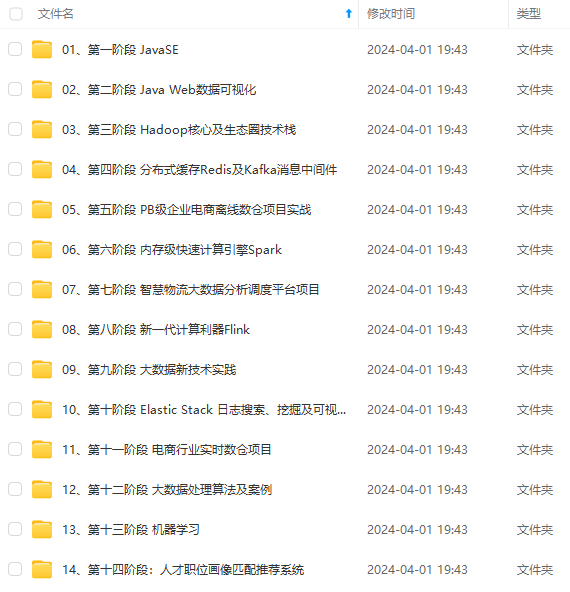
**既有适合小白学习的零基础资料,也有适合3年以上经验的小伙伴深入学习提升的进阶课程,涵盖了95%以上大数据知识点,真正体系化!**
**由于文件比较多,这里只是将部分目录截图出来,全套包含大厂面经、学习笔记、源码讲义、实战项目、大纲路线、讲解视频,并且后续会持续更新**
**[需要这份系统化资料的朋友,可以戳这里获取](https://bbs.csdn.net/topics/618545628)**
45: FutureWarning: The default value of n_estimators will change from 10 in version 0.20 to 100 in 0.22.
"10 in version 0.20 to 100 in 0.22.", FutureWarning)
RandomForestClassifier(bootstrap=True, class_weight=None, criterion='gini',
max_depth=None, max_features='auto', max_leaf_nodes=None,
min_impurity_decrease=0.0, min_impurity_split=None,
min_samples_leaf=1, min_samples_split=2,
min_weight_fraction_leaf=0.0, n_estimators=10,
[外链图片转存中...(img-FfCVzH8u-1714417950844)]
[外链图片转存中...(img-Ore4D1bg-1714417950844)]
[外链图片转存中...(img-B2WZTkd8-1714417950844)]
**既有适合小白学习的零基础资料,也有适合3年以上经验的小伙伴深入学习提升的进阶课程,涵盖了95%以上大数据知识点,真正体系化!**
**由于文件比较多,这里只是将部分目录截图出来,全套包含大厂面经、学习笔记、源码讲义、实战项目、大纲路线、讲解视频,并且后续会持续更新**
**[需要这份系统化资料的朋友,可以戳这里获取](https://bbs.csdn.net/topics/618545628)**

魔乐社区(Modelers.cn) 是一个中立、公益的人工智能社区,提供人工智能工具、模型、数据的托管、展示与应用协同服务,为人工智能开发及爱好者搭建开放的学习交流平台。社区通过理事会方式运作,由全产业链共同建设、共同运营、共同享有,推动国产AI生态繁荣发展。
更多推荐


 12
12 0
0- 0


 已为社区贡献4条内容

所有评论(0)