机器学习 | 基于knn算法求pr曲线和roc曲线
目录
一、引言
模型评估是机器学习不可或缺的一环。在分类问题中,我们通常希望了解模型的预测能力,也就是评估该模型对正类别和负类别的分类结果。PR曲线和ROC曲线是用于评估二分类模型性能的重要工具,通过在不同阈值下的精确度、召回率和真正率、假正率之间的权衡,评估模型的性能。它们可以帮助我们在不同阈值下比较模型的性能,并选择最佳的阈值进行预测。本篇文章将通过KNN模型的PR和ROC曲线绘制,来展示如何进行模型性能评估。
二、KNN模型PR和ROC曲线绘制

2.1PR曲线
2.1.1基本概念
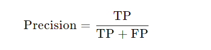
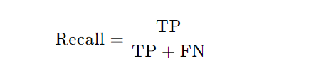
PR曲线是一种用于评估二分类模型性能的图形工具。该曲线有两个重要指标:精确度(Precision)和召回率(Recall)。
精确度:模型预测为正的样本中,实际为正的比例。
计算公式:
召回率:实际为正的样本中,被模型正确预测为正的比例。
计算公式:
2.1.2PR曲线绘制步骤
PR曲线的横坐标为召回率R,纵坐标为精确率P
- 将预测结果按照预测为正类概率值排序
- 将阈值由1开始逐渐降低,按此顺序逐个把样本作为正例进行预测,每次可以计算出当前的P,R值
- 以P为纵坐标,R为横坐标绘制图像
2.1.3PR曲线代码
import numpy as np
import matplotlib.pyplot as plt
from sklearn.model_selection import train_test_split
from sklearn.preprocessing import StandardScaler
from sklearn.neighbors import KNeighborsClassifier

from sklearn.metrics import roc_auc_score


# 生成包含1000个样本的随机数据集
np.random.seed(0)
X = np.random.rand(1000, 10)
y = (X[:, 0] + X[:, 1] > 1).astype(int)

# 划分数据集为训练集和测试集
X_train, X_test, y_train, y_test = train_test_split(X, y, test_size=0.2, random_state=42)

# 特征标准化
scaler = StandardScaler()
X_train = scaler.fit_transform(X_train)
X_test = scaler.transform(X_test)

# 初始化KNN分类器并选择K值
k = 5
knn_classifier = KNeighborsClassifier(n_neighbors=k)

# 训练KNN分类器
knn = KNeighborsClassifier(n_neighbors=5)
knn.fit(X_train, y_train)

# 模型的概率预测
y_scores = knn.predict_proba(X_test)[:, 1]

# 初始化空列表来存储P-R曲线上的点
precision_points = []
recall_points = []

# 遍历不同的阈值
thresholds = np.linspace(0, 1, 10)  # 生成100个阈值
for threshold in thresholds:
    y_pred = (y_scores >= threshold).astype(int)
    # print("y_pred:",y_pred)
    TP = np.sum((y_pred == 1) & (y_test == 1))
    FP = np.sum((y_pred == 1) & (y_test == 0))
    TN = np.sum((y_pred == 0) & (y_test == 0))
    FN = np.sum((y_pred == 0) & (y_test == 1))
    precision = TP / (TP + FP) if TP + FP > 0 else 1.0
    recall = TP / (TP + FN) if TP + FN > 0 else 1.0
    precision_points.append(precision)
    recall_points.append(recall)

print("TP:", TP)
print("FP:", FP)
print("TN:", TN)
print("FN:", FN)
print("R:", recall_points)
print("P:", precision_points)

# 绘制PR曲线
plt.plot(recall_points, precision_points, marker='.')
plt.xlabel('Recall')
plt.ylabel('Precision')
plt.title('PR Curve')
plt.grid(True)
plt.show()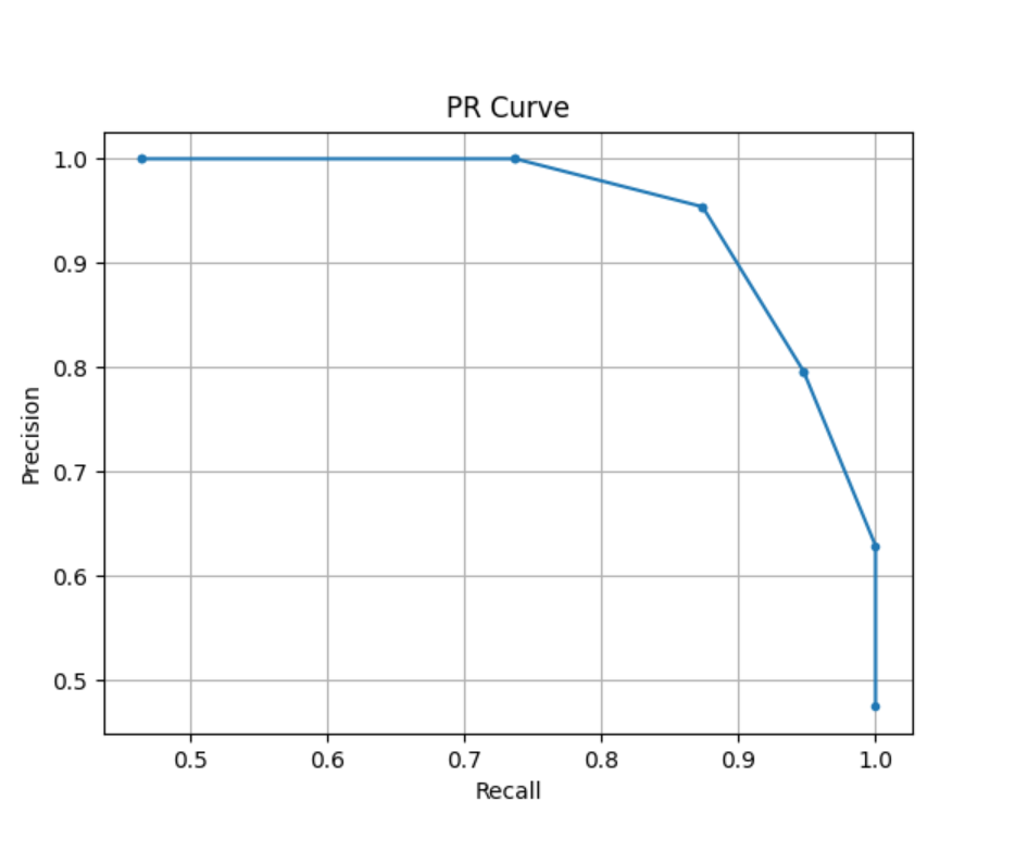
2.2ROC曲线
2.2.1基本概念
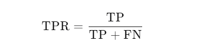
ROC曲线通常用于评估二元分类器,用于可视化分类器在不同阈值下的性能表现。该曲线的两个重要指标:真正例率(TPR)和假正例率(FPR)。ROC曲线的目标是在各种不同阈值下,找到一个平衡点,使FPR尽可能低,而TPR尽可能高。
TPR:真正例率是实际为正的样本中,被模型正确预测为正的比例。
计算公式:
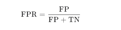
FPR:假正例率是实际为负的样本中,被模型错误预测为正的比例。
计算公式:
2.2.2ROC曲线绘制步骤
1.假设已经得出一系列样本被划分为正类的概率Score值,按照大小排序。
2.从高到低,依次将“Score”值作为阈值threshold,当测试样本属于正样本的概率大于或等于这个threshold时,我们认为它为正样本,否则为负样本。举例来说,对于某个样本,其“Score”值为0.6,那么“Score”值大于等于0.6的样本都被认为是正样本,而其他样本则都认为是负样本。
3.每次选取一个不同的threshold,得到一组FPR和TPR,以FPR值为横坐标和TPR值为纵坐标,即ROC曲线上的一点。
4.根据3中的每个坐标点,画图。
2.2.3ROC曲线代码
import numpy as np
import matplotlib.pyplot as plt
from sklearn.model_selection import train_test_split
from sklearn.preprocessing import StandardScaler
from sklearn.neighbors import KNeighborsClassifier

from sklearn.metrics import roc_auc_score


# 生成包含1000个样本的随机数据集
np.random.seed(0)
X = np.random.rand(1000, 10)
y = (X[:, 0] + X[:, 1] > 1).astype(int)

# 划分数据集为训练集和测试集
X_train, X_test, y_train, y_test = train_test_split(X, y, test_size=0.2, random_state=42)

# 特征标准化
scaler = StandardScaler()
X_train = scaler.fit_transform(X_train)
X_test = scaler.transform(X_test)

# 初始化KNN分类器并选择K值
k = 5
knn_classifier = KNeighborsClassifier(n_neighbors=k)

# 训练KNN分类器
knn = KNeighborsClassifier(n_neighbors=5)
knn.fit(X_train, y_train)

# 模型的概率预测
y_scores = knn.predict_proba(X_test)[:, 1]

# 初始化空列表来存储P-R曲线上的点
TPR_points = []
FPR_points = []

# 遍历不同的阈值
thresholds = np.linspace(0, 1, 10)  # 生成100个阈值
for threshold in thresholds:
    y_pred = (y_scores >= threshold).astype(int)
    TP = np.sum((y_pred == 1) & (y_test == 1))
    FP = np.sum((y_pred == 1) & (y_test == 0))
    TN = np.sum((y_pred == 0) & (y_test == 0))
    FN = np.sum((y_pred == 0) & (y_test == 1))
    TPR = TP / (TP + FN)
    FPR = FP / (FP + TN)
    TPR_points.append(TPR)
    FPR_points.append(FPR)

print("TP:", TP)
print("FP:", FP)
print("TN:", TN)
print("FN:", FN)
print("FPR:", FPR_points)
print("TPR:", TPR_points)

# 计算AUC
# 计算 ROC AUC
roc_auc = roc_auc_score(y_test, y_scores)
print("AUC = ", roc_auc)

# 绘制 ROC 曲线
plt.figure()
plt.plot(FPR_points, TPR_points, color='darkorange', lw=2)
plt.plot([0, 1], [0, 1], color='navy', lw=2, linestyle='--')
plt.xlim([0.0, 1.0])
plt.ylim([0.0, 1.05])
plt.xlabel('FPR')
plt.ylabel('TPR')
plt.title('ROC')
plt.show()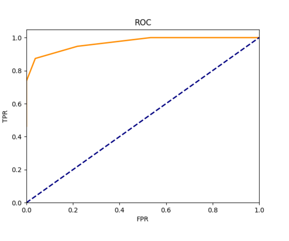

魔乐社区(Modelers.cn) 是一个中立、公益的人工智能社区,提供人工智能工具、模型、数据的托管、展示与应用协同服务,为人工智能开发及爱好者搭建开放的学习交流平台。社区通过理事会方式运作,由全产业链共同建设、共同运营、共同享有,推动国产AI生态繁荣发展。
更多推荐


 12
12 0
0- 0


 已为社区贡献2条内容

所有评论(0)