最详细吴恩达机器学习课后作业(2):Logistic regression(文末有完整代码copy)
Logistic regression在这部分的练习中,你将建立一个逻辑回归模型来预测一个学生是否能进入大学。假设你是一所大学的行政管理人员,你想根据两门考试的结果,来决定每个申请人是否被录取。你有以前申请人的历史数据,可以将其用作逻辑回归训练集。对于每一个训练样本,你有申请人两次测评的分数以及录取的结果。为了完成这个预测任务,我们准备构建一个可以基于两次测试评分来评估录取可能性的分类模型。Pre
Logistic regression
在这部分的练习中,你将建立一个逻辑回归模型来预测一个学生是否能进入大学。假设你是一所大学的行政管理人员,你想根据两门考试的结果,来决定每个申请人是否被录取。你有以前申请人的历史数据,可以将其用作逻辑回归训练集。对于每一个训练样本,你有申请人两次测评的分数以及录取的结果。为了完成这个预测任务,我们准备构建一个可以基于两次测试评分来评估录取可能性的分类模型。
Prepare datasets
import numpy as np
import pandas as pd
import matplotlib.pyplot as plt
import scipy.optimize as opt
'''
1.Prepare datasets
'''
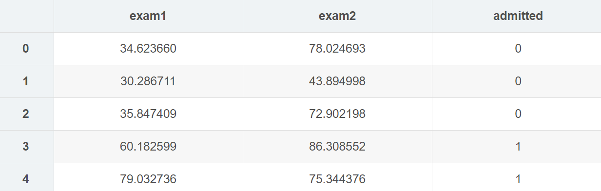
data = pd.read_csv('ex2data1.txt', names=['exam1', 'exam2', 'admitted'])
data.head()
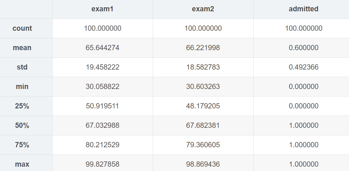
data.describe()
分类数据,将录取和未录取分开
positive = data[data.admitted.isin([1])]  # 1
negetive = data[data.admitted.isin([0])]  # 0
可视化图形,得到一个大概对数据的了解
fig, ax = plt.subplots(figsize=(6, 5))
ax.scatter(positive['exam1'], positive['exam2'], c='orange', label='Admitted')
ax.scatter(negetive['exam1'], negetive['exam2'], c='b', marker='*', label='Not Admitted')
# 设置图例显示在图的上方
box = ax.get_position()
# 若是将图例画在坐标外边,如果放在右边,一般要给width*0.8左右的值,在上边,要给height*0.8左右的值
ax.set_position([box.x0, box.y0, box.width, box.height*0.8])
ax.legend(loc='center left', bbox_to_anchor=(0.2, 1.12), ncol=2)
'''
(横向看右,纵向看下),如果要自定义图例位置或者将图例画在坐标外边,用它,
比如bbox_to_anchor=(1.4,0.8),这个一般配合着ax.get_position(),set_position([box.x0, box.y0, box.width*0.8 , box.height])使用
用不到的参数可以直接去掉,有的参数没写进去,用得到的话加进去 , bbox_to_anchor=(1.11,0)
‘’’
'''
# 设置横纵坐标名
ax.set_xlabel('Exam 1 Score')
ax.set_ylabel('Exam 2 Score')
# plt.show()
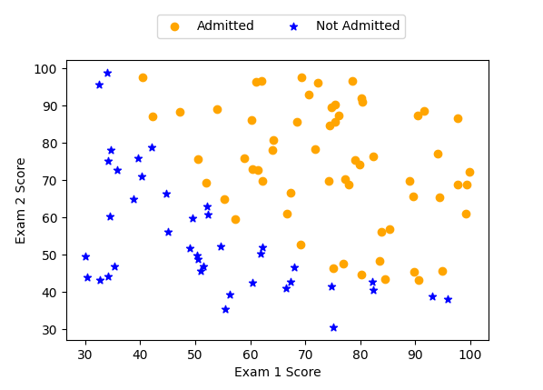
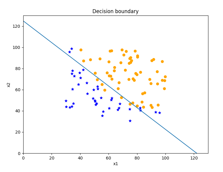
看起来在两类间,有一个清晰的决策边界。现在我们需要实现逻辑回归,那样就可以训练一个模型来预测结果。
根据输入和输出对相应的数据进行调整
# 根据相关的X矩阵对数据进行一下处理
if 'Ones' not in data.columns:
    data.insert(0, 'Ones', 1)
    pass

# 设置相对应的X(training data)和y(target variable),统一使用矩阵/数组,又是矩阵又是数组很容易出错
# https://zhuanlan.zhihu.com/p/46056842,记住矩阵和数组的使用方法,只用数组来进行计算
# np.dot()函数:对于秩为1的数组,执行对应位置相乘,然后再相加;对于秩不为1的二维数组,执行矩阵乘法运算
X = np.array(data.iloc[:, :-1])
y = np.array(data.iloc[:, -1])
theta = np.zeros(X.shape[1])
print(X.shape, y.shape, theta.shape)
Design model using gradient descend
1. Sigmoid function
首先来回顾下 logistic回归的假设函数:
hθ(x)=g(θTx)=11+e−θTX h_{\theta}(x)=g\left(\theta^{T} x\right)=\frac{1}{1+e^{-\theta^{T} X}} hθ(x)=g(θTx)=1+e−θTX1
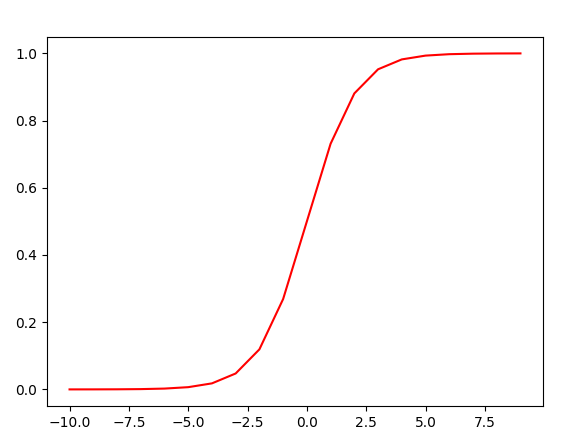
其中的 g代表一个常用的logistic function为S形函数 (Sigmoid function) :
g(z)=11+e−z g(z)=\frac{1}{1+e^{-z}} g(z)=1+e−z1
# 1)Sigmoid Fuc
def sigmoid(z):
    return 1 / (1 + np.exp(-z))
测试一下,此函数是否是对的
# 测试一下,保证Sigmoid函数正确性
x1 = np.arange(-10, 10, 1)
plt.plot(x1, sigmoid(x1), c='r')
# plt.show()
2. Cost Function
逻辑回归的代价函数如下, 和线性回归的代价函数不一样, 因为这个函数是凸的。
J(θ)=1m∑i=1m[−y(i)log(hθ(x(i)))−(1−y(i))log(1−hθ(x(i)))]hθ(x)=g(θTx) \begin{array}{c} J(\theta)=\frac{1}{m} \sum_{i=1}^{m}\left[-y^{(i)} \log \left(h_{\theta}\left(x^{(i)}\right)\right)-\left(1-y^{(i)}\right) \log \left(1-h_{\theta}\left(x^{(i)}\right)\right)\right] \\ h_{\theta}(x)=g\left(\theta^{T} x\right) \end{array} J(θ)=m1∑i=1m[−y(i)log(hθ(x(i)))−(1−y(i))log(1−hθ(x(i)))]hθ(x)=g(θTx)
# 2)Cost Fuc
def cost(theta, X, y):
    first = (-y) * np.log(sigmoid(X @ theta))
    second = (1 - y)*np.log(1 - sigmoid(X @ theta))
    return np.mean(first - second)
# 测试一下cost,进行向量化的时候一定要找准对应关系
a = cost(theta, X, y)   # 0.6931471805599453
3. Gradient function
这是批量梯度下降 (batch gradient descent)
转化为向量化计算: 1mXT(Sigmoid(Xθ)−y)\frac{1}{m} X^{T}(\operatorname{Sigmoid}(X \theta)-y)m1XT(Sigmoid(Xθ)−y)
∂J(θ)∂θj=1m∑i=1m(hθ(x(i))−y(i))xj(i) \frac{\partial J(\theta)}{\partial \theta_{j}}=\frac{1}{m} \sum_{i=1}^{m}\left(h_{\theta}\left(x^{(i)}\right)-y^{(i)}\right) x_{j}^{(i)} ∂θj∂J(θ)=m1i=1∑m(hθ(x(i))−y(i))xj(i)
# 3)Gradient Fuc
'''
batch gradient descent
转为向量化计算
'''


def gradient(theta, X, y):
    # the gradient of the cost is a vector of the same length as θ where the jth element (for j = 0, 1, . . . , n)
    return (X.T @ (sigmoid(X @ theta) - y)) / len(X)
# @相当于.dot()

print(gradient(theta, X, y))
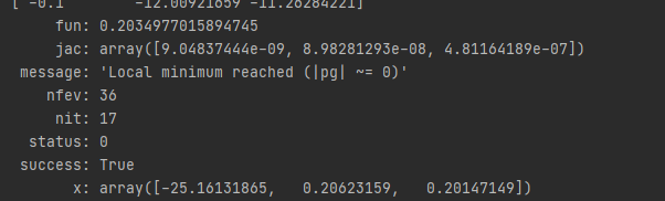
4. Optimization
我们实际上没有在这个函数中执行梯度下降,我们仅仅在计算梯度。在练习中,一个称为“fminunc”的Octave函数是用来优化函数来计算成本和梯度参数。由于我们使用Python,我们可以用SciPy的“optimize”命名空间来做同样的事情。
这里我们使用的是高级优化算法,运行速度通常远远超过梯度下降。方便快捷。
只需传入cost函数,已经所求的变量theta,和梯度。cost函数定义变量时变量tehta要放在第一个,若cost函数只返回cost,则设置fprime=gradient。
import scipy.optimize as opt
res = opt.minimize(fun=cost, x0=theta, jac=gradient, args=(X, y), method='TNC')
# res2 = opt.fmin_tnc(func=cost, x0=theta, fprime=gradient, args=(X, y))
print(res)
# 有两种方法可以用来实现优化,找到最终的theta
Run model
逻辑回归模型的假设函数:
hθ(x)=11+e−θTX h_{\theta}(x)=\frac{1}{1+e^{-\theta^{T} X}} hθ(x)=1+e−θTX1
def predict(theta, X):
    probability = sigmoid(X @ theta)
    return [1 if x >= 0.5 else 0 for x in probability]  # return a list


# learning_parameters = np.array([-25.1613186, 0.20623159, 0.20147149])
predictions = predict(res.x, X)
print(predictions)
correct = []
for i in range(len(predictions)):
    if predictions[i] == y[i]:
        correct.append(1)
    else:
        correct.append(0)
        pass
    pass
# correct = [1 if a == b else 0 for (a, b) in zip(predictions, y)] 这样也可以返回一个list
accuracy = sum(correct)/len(X)
print(accuracy)

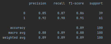
1. sklearn中的方法来检验
'''
4.sklearn中的方法来检验
'''
from sklearn.metrics import classification_report
print(classification_report(predictions, y))
Decision boundary
X×θ=0 (this is the line) θ0+x1θ1+x2θ2=0 \begin{array}{l} X \times \theta=0 \text { (this is the line) }\\ \theta_{0}+x_{1} \theta_{1}+x_{2} \theta_{2}=0 \end{array} X×θ=0 (this is the line) θ0+x1θ1+x2θ2=0
# 以下是根据数学关系式来决定的
x1 = np.arange(130, step=0.1)
x2 = -(res.x[0] + x1 * res.x[1]) / res.x[2]

fig2, ax = plt.subplots(figsize=(8, 6))
ax.scatter(positive['exam1'], positive['exam2'], c='orange', label='Admitted')
ax.scatter(negetive['exam1'], negetive['exam2'], c='b', marker='*', label='Not Admitted')
ax.plot(x1, x2)
ax.set_xlim(0, 130)
ax.set_ylim(0, 130)
ax.set_xlabel('x1')
ax.set_ylabel('x2')
ax.set_title('Decision boundary')
plt.show()
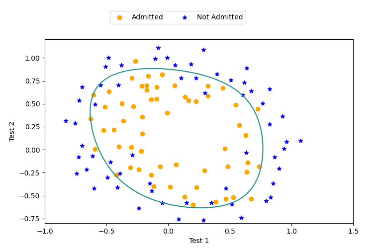
Regularized logistic regression
我们将要通过加入正则项提升逻辑回归算法。简而言之,正则化是成本函数中的一个术语,它使算法更倾向于“更简单”的模型(在这种情况下,模型将更小的系数)。这个理论助于减少过拟合,提高模型的泛化能力。这样,我们开始吧。
设想你是工厂的生产主管,你有一些芯片在两次测试中的测试结果。对于这两次测试,你想决定是否芯片要被接受或抛弃。为了帮助你做出艰难的决定,你拥有过去芯片的测试数据集,从其中你可以构建一个逻辑回归模型。
声明:该部分只会把和上述实现代码方式的不同方法展现出来,其他部分不作额外的说明
Prepare Datasets
data2 = pd.read_csv('ex2data2.txt', names=['Test 1', 'Test 2', 'Accepted'])
print(data2.head())


# 可视化已有数据
def plotData():
    # 分类数据,将录取和未录取分开
    positive = data2[data2.Accepted.isin([1])]  # 1
    negetive = data2[data2.Accepted.isin([0])]  # 0

    fig, ax = plt.subplots(figsize=(8, 6))
    ax.scatter(positive['Test 1'], positive['Test 2'], c='orange', label='Admitted')
    ax.scatter(negetive['Test 1'], negetive['Test 2'], c='b', marker='*', label='Not Admitted')
    # 设置图例显示在图的上方
    box = ax.get_position()
    # 若是将图例画在坐标外边,如果放在右边,一般要给width*0.8左右的值,在上边,要给height*0.8左右的值
    ax.set_position([box.x0, box.y0, box.width, box.height * 0.8])
    ax.legend(loc='center left', bbox_to_anchor=(0.2, 1.12), ncol=2)
    '''
    (横向看右,纵向看下),如果要自定义图例位置或者将图例画在坐标外边,用它,
    比如bbox_to_anchor=(1.4,0.8),这个一般配合着ax.get_position(),set_position([box.x0, box.y0, box.width*0.8 , box.height])使用
    用不到的参数可以直接去掉,有的参数没写进去,用得到的话加进去 , bbox_to_anchor=(1.11,0)
    ‘’’
    '''
    # 设置横纵坐标名
    ax.set_xlabel('Test 1')
    ax.set_ylabel('Test 2')
    # plt.show()
    pass
Feature mapping(特征缩放)
一个拟合数据的更好的方法是从每个数据点创建更多的特征。
我们将把这些特征映射到所有的x1和x2的多项式项上;
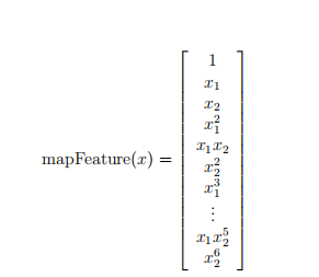
def featureMapping(x1, x2, power):
    data = {}
    # data此处是一个字典
    for i in np.arange(power + 1):
        for p in np.arange(i + 1):
            data["f{}{}".format(i - p, p)] = np.power(x1, i-p) * np.power(x2, p)
            pass
    # 假设power=3,则字典中会形成00,10,01,20,11,02,30,21,12,03列数据
    return pd.DataFrame(data)
查看缩放数据
x1 = np.array(data2['Test 1'])
x2 = np.array(data2['Test 2'])

_data2 = featureMapping(x1, x2, 7)
# print(_data2)
[外链图片转存失败,源站可能有防盗链机制,建议将图片保存下来直接上传(img-WYhw4AGe-1622168525288)(C:\Users\DELL\AppData\Roaming\Typora\typora-user-images\image-20210528101425097.png)]
经过映射,我们将有两个特征的向量转化成了一个36维的向量。
在这个高维特征向量上训练的logistic回归分类器将会有一个更复杂的决策边界,当我们在二维图中绘制时,会出现非线性。
虽然特征映射允许我们构建一个更有表现力的分类器,但它也更容易过拟合。在接下来的练习中,我们将实现正则化的logistic回归来拟合数据,并且可以看到正则化如何帮助解决过拟合的问题。
处理数据
# 先获取特征,标签以及参数theta,确保维度良好
X = np.array(_data2)
y = np.array(data2['Accepted'])
theta = np.zeros(X.shape[1])
print(X.shape, y.shape, theta.shape)
Regularized Cost Funciton
J(θ)=1m∑i=1m[−y(i)log(hθ(x(i)))−(1−y(i))log(1−hθ(x(i)))]+λ2m∑j=1nθj2 J(\theta)=\frac{1}{m} \sum_{i=1}^{m}\left[-y^{(i)} \log \left(h_{\theta}\left(x^{(i)}\right)\right)-\left(1-y^{(i)}\right) \log \left(1-h_{\theta}\left(x^{(i)}\right)\right)\right]+\frac{\lambda}{2 m} \sum_{j=1}^{n} \theta_{j}^{2} J(θ)=m1i=1∑m[−y(i)log(hθ(x(i)))−(1−y(i))log(1−hθ(x(i)))]+2mλj=1∑nθj2
注意:不惩罚第一项 θ0\theta_{0}θ0
实现代码如下:
# 1)Sigmoid Fuc
def sigmoid(z):
    return 1 / (1 + np.exp(-z))


# 2)Cost Fuc
def cost(theta, X, y):
    first = (-y) * np.log(sigmoid(X @ theta))
    second = (1 - y)*np.log(1 - sigmoid(X @ theta))
    return np.mean(first - second)


def gradient(theta, X, y):
    # the gradient of the cost is a vector of the same length as θ where the jth element (for j = 0, 1, . . . , n)
    return (X.T @ (sigmoid(X @ theta) - y)) / len(X)


def costReg(theta, X, y, Lambda):
    # 不惩罚第一项(去掉第0项)
    _theta = theta[1:]
    reg = (Lambda/2*len(X))*(_theta @ _theta)   # _theta@_theta == inner product
    return cost(theta, X, y) + reg


a = costReg(theta, X, y, 1)     # 0.6931471805599454 此时θ均为0


def gradientReg(theta, X, y, Lambda):
    reg = (Lambda/len(X)) * theta
    reg[0] = 0
    return gradient(theta, X, y) + reg


b = gradientReg(theta, X, y, 1)
# print(b)


def predict(theta, X):
    probability = sigmoid(X @ theta)
    return [1 if x >= 0.5 else 0 for x in probability]  # return a list
Optimization
# res = opt.fmin_tnc(func=costReg, x0=theta, fprime=gradientReg, args=(X, y, 2))
res = opt.minimize(fun=costReg, x0=theta, jac=gradientReg, args=(X, y, 1), method='TNC')
# print(res)

from sklearn import linear_model    # 调用sklearn的线性回归包
model = linear_model.LogisticRegression(penalty='l2', C=1.0)
model.fit(X, y.ravel())
# print(model.score(X, y))    # 0.8305084745762712
后面和练习2的第一题一致
'''
-Evaluating logistic regression
'''
final_theta = res.x
predictions = predict(final_theta, X)
correct = [1 if a == b else 0 for (a, b) in zip(predictions, y)]
accuracy = sum(correct) / len(correct)
print(accuracy)

# 或者用sklearn中的方法来评估结果。
from sklearn.metrics import classification_report
print(classification_report(y, predictions))


'''
-Decision boundary
'''
x = np.linspace(-1, 1.5, 150)
xx, yy = np.meshgrid(x, x)
# 生成由x组成的网格图 横坐标x和纵坐标y经过meshgrid(x,y)后返回了所有直线相交的网络坐标点的横坐标xx和纵坐标yy  150,150
# xx.ravel()转换成一维数据
z = np.array(featureMapping(xx.ravel(), yy.ravel(), 7))

z = z @ final_theta
z = z.reshape(xx.shape)

plotData()
plt.contour(xx, yy, z, 0)
plt.ylim(-0.8, 1.2)
plt.show()
最后附上两次练习的完整代码
import numpy as np
import pandas as pd
import matplotlib.pyplot as plt
import scipy.optimize as opt

'''
1.Prepare datasets
'''

data = pd.read_csv('ex2data1.txt', names=['exam1', 'exam2', 'admitted'])
data.head()
data.describe()

# 分类数据,将录取和未录取分开
positive = data[data.admitted.isin([1])]  # 1
negetive = data[data.admitted.isin([0])]  # 0

fig, ax = plt.subplots(figsize=(6, 5))
ax.scatter(positive['exam1'], positive['exam2'], c='orange', label='Admitted')
ax.scatter(negetive['exam1'], negetive['exam2'], c='b', marker='*', label='Not Admitted')
# 设置图例显示在图的上方
box = ax.get_position()
# 若是将图例画在坐标外边,如果放在右边,一般要给width*0.8左右的值,在上边,要给height*0.8左右的值
ax.set_position([box.x0, box.y0, box.width, box.height*0.8])
ax.legend(loc='center left', bbox_to_anchor=(0.2, 1.12), ncol=2)
'''
(横向看右,纵向看下),如果要自定义图例位置或者将图例画在坐标外边,用它,
比如bbox_to_anchor=(1.4,0.8),这个一般配合着ax.get_position(),set_position([box.x0, box.y0, box.width*0.8 , box.height])使用
用不到的参数可以直接去掉,有的参数没写进去,用得到的话加进去 , bbox_to_anchor=(1.11,0)
‘’’
'''
# 设置横纵坐标名
ax.set_xlabel('Exam 1 Score')
ax.set_ylabel('Exam 2 Score')
# plt.show()

# 根据相关的X矩阵对数据进行一下处理
if 'Ones' not in data.columns:
    data.insert(0, 'Ones', 1)
    pass

# 设置相对应的X(training data)和y(target variable),统一使用矩阵/数组,又是矩阵又是数组很容易出错
# https://zhuanlan.zhihu.com/p/46056842,记住矩阵和数组的使用方法,只用数组来进行计算
# np.dot()函数:对于秩为1的数组,执行对应位置相乘,然后再相加;对于秩不为1的二维数组,执行矩阵乘法运算
X = np.array(data.iloc[:, :-1])
y = np.array(data.iloc[:, -1])
theta = np.zeros(X.shape[1])
print(X.shape, y.shape, theta.shape)

'''
2.Design model using gradient descend
'''


# 1)Sigmoid Fuc
def sigmoid(z):
    return 1 / (1 + np.exp(-z))


# 测试一下,保证Sigmoid函数正确性
x1 = np.arange(-10, 10, 1)
plt.plot(x1, sigmoid(x1), c='r')
# plt.show()


# 2)Cost Fuc
def cost(theta, X, y):
    first = (-y) * np.log(sigmoid(X @ theta))
    second = (1 - y)*np.log(1 - sigmoid(X @ theta))
    return np.mean(first - second)


# 测试一下cost,进行向量化的时候一定要找准对应关系
a = cost(theta, X, y)   # 0.6931471805599453

# 3)Gradient Fuc
'''
batch gradient descent
转为向量化计算
'''


def gradient(theta, X, y):
    # the gradient of the cost is a vector of the same length as θ where the jth element (for j = 0, 1, . . . , n)
    return (X.T @ (sigmoid(X @ theta) - y)) / len(X)


print(gradient(theta, X, y))

res = opt.minimize(fun=cost, x0=theta, jac=gradient, args=(X, y), method='TNC')
# res2 = opt.fmin_tnc(func=cost, x0=theta, fprime=gradient, args=(X, y))
print(res)

'''
3.Run model
'''


def predict(theta, X):
    probability = sigmoid(X @ theta)
    return [1 if x >= 0.5 else 0 for x in probability]  # return a list


# learning_parameters = np.array([-25.1613186, 0.20623159, 0.20147149])
predictions = predict(res.x, X)
print(predictions)
correct = []
for i in range(len(predictions)):
    if predictions[i] == y[i]:
        correct.append(1)
    else:
        correct.append(0)
        pass
    pass
# correct = [1 if a == b else 0 for (a, b) in zip(predictions, y)] 这样也可以返回一个list
accuracy = sum(correct)/len(X)
print(accuracy)


'''
4.sklearn中的方法来检验
'''
from sklearn.metrics import classification_report
print(classification_report(predictions, y))


'''
5.Decision boundary
'''
# 以下是根据数学关系式来决定的
x1 = np.arange(130, step=0.1)
x2 = -(res.x[0] + x1 * res.x[1]) / res.x[2]

fig2, ax = plt.subplots(figsize=(8, 6))
ax.scatter(positive['exam1'], positive['exam2'], c='orange', label='Admitted')
ax.scatter(negetive['exam1'], negetive['exam2'], c='b', marker='*', label='Not Admitted')
ax.plot(x1, x2)
ax.set_xlim(0, 130)
ax.set_ylim(0, 130)
ax.set_xlabel('x1')
ax.set_ylabel('x2')
ax.set_title('Decision boundary')
plt.show()
import numpy as np
import pandas as pd
import matplotlib.pyplot as plt
import scipy.optimize as opt

data2 = pd.read_csv('ex2data2.txt', names=['Test 1', 'Test 2', 'Accepted'])
print(data2.head())


# 可视化已有数据
def plotData():
    # 分类数据,将录取和未录取分开
    positive = data2[data2.Accepted.isin([1])]  # 1
    negetive = data2[data2.Accepted.isin([0])]  # 0

    fig, ax = plt.subplots(figsize=(8, 6))
    ax.scatter(positive['Test 1'], positive['Test 2'], c='orange', label='Admitted')
    ax.scatter(negetive['Test 1'], negetive['Test 2'], c='b', marker='*', label='Not Admitted')
    # 设置图例显示在图的上方
    box = ax.get_position()
    # 若是将图例画在坐标外边,如果放在右边,一般要给width*0.8左右的值,在上边,要给height*0.8左右的值
    ax.set_position([box.x0, box.y0, box.width, box.height * 0.8])
    ax.legend(loc='center left', bbox_to_anchor=(0.2, 1.12), ncol=2)
    '''
    (横向看右,纵向看下),如果要自定义图例位置或者将图例画在坐标外边,用它,
    比如bbox_to_anchor=(1.4,0.8),这个一般配合着ax.get_position(),set_position([box.x0, box.y0, box.width*0.8 , box.height])使用
    用不到的参数可以直接去掉,有的参数没写进去,用得到的话加进去 , bbox_to_anchor=(1.11,0)
    ‘’’
    '''
    # 设置横纵坐标名
    ax.set_xlabel('Test 1')
    ax.set_ylabel('Test 2')
    # plt.show()
    pass


# plotData()

'''
-Feature mapping
'''

def featureMapping(x1, x2, power):
    data = {}
    # data此处是一个字典
    for i in np.arange(power + 1):
        for p in np.arange(i + 1):
            data["f{}{}".format(i - p, p)] = np.power(x1, i-p) * np.power(x2, p)
            pass
    # 假设power=3,则字典中会形成00,10,01,20,11,02,30,21,12,03列数据
    return pd.DataFrame(data)


x1 = np.array(data2['Test 1'])
x2 = np.array(data2['Test 2'])

_data2 = featureMapping(x1, x2, 7)
# print(_data2)

'''
-Regularized Cost Fuc
'''
# 先获取特征,标签以及参数theta,确保维度良好
X = np.array(_data2)
y = np.array(data2['Accepted'])
theta = np.zeros(X.shape[1])
print(X.shape, y.shape, theta.shape)


# 1)Sigmoid Fuc
def sigmoid(z):
    return 1 / (1 + np.exp(-z))


# 2)Cost Fuc
def cost(theta, X, y):
    first = (-y) * np.log(sigmoid(X @ theta))
    second = (1 - y)*np.log(1 - sigmoid(X @ theta))
    return np.mean(first - second)


def gradient(theta, X, y):
    # the gradient of the cost is a vector of the same length as θ where the jth element (for j = 0, 1, . . . , n)
    return (X.T @ (sigmoid(X @ theta) - y)) / len(X)


def costReg(theta, X, y, Lambda):
    # 不惩罚第一项(去掉第0项)
    _theta = theta[1:]
    reg = (Lambda/2*len(X))*(_theta @ _theta)   # _theta@_theta == inner product
    return cost(theta, X, y) + reg


a = costReg(theta, X, y, 1)     # 0.6931471805599454 此时θ均为0


def gradientReg(theta, X, y, Lambda):
    reg = (Lambda/len(X)) * theta
    reg[0] = 0
    return gradient(theta, X, y) + reg


b = gradientReg(theta, X, y, 1)
# print(b)


def predict(theta, X):
    probability = sigmoid(X @ theta)
    return [1 if x >= 0.5 else 0 for x in probability]  # return a list


'''
-其他方法
'''
# res = opt.fmin_tnc(func=costReg, x0=theta, fprime=gradientReg, args=(X, y, 2))
res = opt.minimize(fun=costReg, x0=theta, jac=gradientReg, args=(X, y, 1), method='TNC')
# print(res)

from sklearn import linear_model    # 调用sklearn的线性回归包
model = linear_model.LogisticRegression(penalty='l2', C=1.0)
model.fit(X, y.ravel())
# print(model.score(X, y))    # 0.8305084745762712

'''
-Evaluating logistic regression
'''
final_theta = res.x
predictions = predict(final_theta, X)
correct = [1 if a == b else 0 for (a, b) in zip(predictions, y)]
accuracy = sum(correct) / len(correct)
print(accuracy)

# 或者用sklearn中的方法来评估结果。
from sklearn.metrics import classification_report
print(classification_report(y, predictions))


'''
-Decision boundary
'''
x = np.linspace(-1, 1.5, 150)
xx, yy = np.meshgrid(x, x)
# 生成由x组成的网格图 横坐标x和纵坐标y经过meshgrid(x,y)后返回了所有直线相交的网络坐标点的横坐标xx和纵坐标yy  150,150
# xx.ravel()转换成一维数据
z = np.array(featureMapping(xx.ravel(), yy.ravel(), 7))

z = z @ final_theta
z = z.reshape(xx.shape)

plotData()
plt.contour(xx, yy, z, 0)
plt.ylim(-0.8, 1.2)
plt.show()
祝大家平安喜乐,健康开心~~
参考文献:https://blog.csdn.net/Cowry5/article/details/80247569

魔乐社区(Modelers.cn) 是一个中立、公益的人工智能社区,提供人工智能工具、模型、数据的托管、展示与应用协同服务,为人工智能开发及爱好者搭建开放的学习交流平台。社区通过理事会方式运作,由全产业链共同建设、共同运营、共同享有,推动国产AI生态繁荣发展。
更多推荐


 6
6 0
0- 0


 已为社区贡献2条内容

所有评论(0)