>- **🍨 本文为[🔗365天深度学习训练营]中的学习记录博客**
>- **🍖 原作者：[K同学啊]**

本人往期文章可查阅： 深度学习总结

🏡 我的环境：

• 语言环境：Python3.11

• 编译器：Jupyter Lab

• 深度学习环境：Pytorch

• • torch==2.0.0+cu118

• • torchvision==0.18.1+cu118
• 显卡：NVIDIA GeForce GTX 1660

一、数据预处理

1. 任务说明

       本次将加入Word2Vec使用PyTorch实现中文文本分类，Word2Vec 则是其中的一种词嵌入方法，是一种用于生成词向量的浅层神经网络模型，由Tomas Mikolov及其团队于2013年提出。Word2Vec通过学习大量文本数据，将每个单词表示为一个连续的向量，这些向量可以捕捉单词之间的语义和句法关系。数据示例如下：

本周任务：

• 1. 结合Word2Vec文本内容（第1列）预测文本标签（第2列）

• 2. 优化本文网络结构，将准确率提升至89%

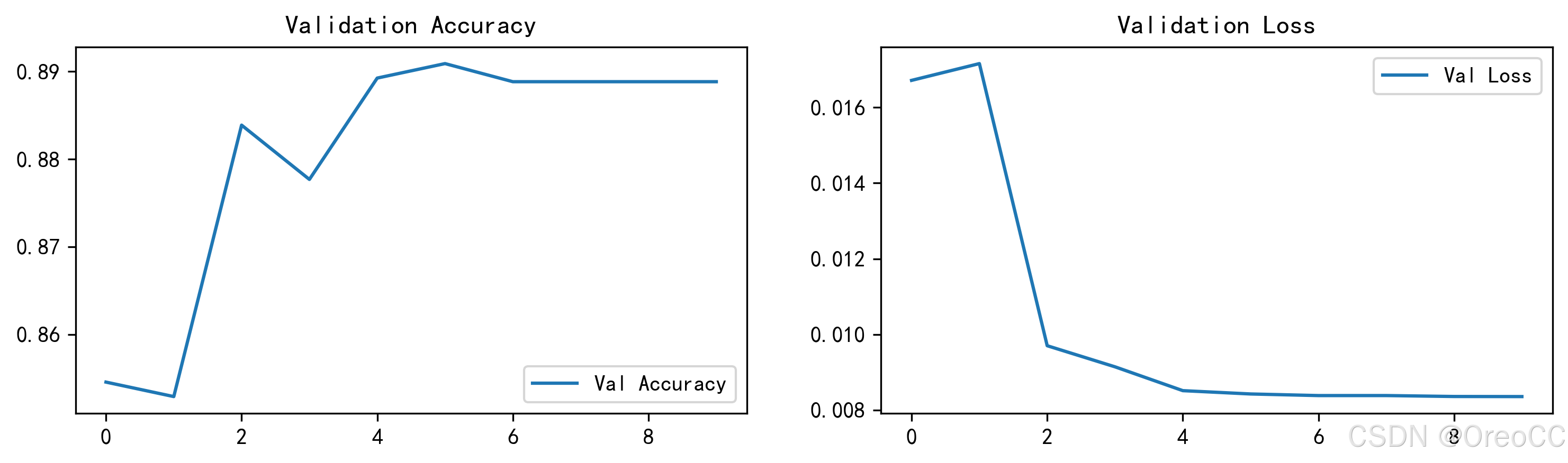
• 3. 绘制出验证集的ACC与Loss图

进阶任务：

• 1. 尝试根据第2周的内容独立实现，尽可能的不看本文的代码

2. 加载数据

import torch
import torch.nn as nn
import torchvision
from torchvision import transforms,datasets
import os,PIL,pathlib,warnings

warnings.filterwarnings("ignore")

device=torch.device("cuda" if torch.cuda.is_available() else "cpu")
device

输出：

device(type='cuda')

import pandas as pd

# 加载自定义中文数据
train_data=pd.read_csv(r'E:/DATABASE/N-series/N8/train.csv',sep='\t',header=None)
train_data.head()

输出：

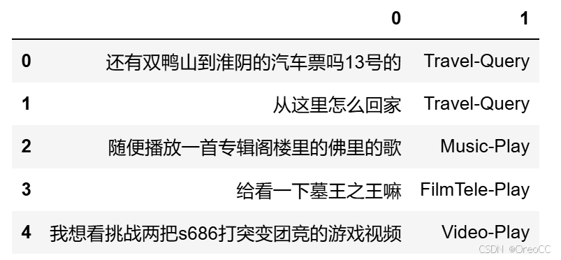
# 构造数据集迭代器
def coustom_data_iter(texts,labels):
    for x,y in zip(texts,labels):
        yield x,y
    
x=train_data[0].values[:]
# 多类标签的one-hot展开
y=train_data[1].values[:]

       zip 是Python中的一个内置函数，它可以将多个序列（列表、元组等）中对应的元素打包成一个个元组，然后返回这些元组组成的一个迭代器。例如，在代码中  zip(texts,labels)  就是将 texts 和 labels 两个列表中对应位置的元素——打包成元组，返回一个迭代器，每次迭代返回一个元组  (x, u)  ，其中 x 是 texts 中的一个元素，y 是 labels 中对应的一个元素。这样，每次从迭代器中获取一个元素，就相当于从 texts 和 labels 中获取了一组对应的数据。在这里，zip 函数主要用于将输入的 texts 和 labels 打包成一个可迭代的数据集，然后传给后续的模型训练过程使用。

查看结果：

x,y

输出：

(array(['还有双鸭山到淮阴的汽车票吗13号的', '从这里怎么回家', '随便播放一首专辑阁楼里的佛里的歌', ...,
        '黎耀祥陈豪邓萃雯畲诗曼陈法拉敖嘉年杨怡马浚伟等到场出席', '百事盖世群星星光演唱会有谁', '下周一视频会议的闹钟帮我开开'],
       dtype=object),
 array(['Travel-Query', 'Travel-Query', 'Music-Play', ..., 'Radio-Listen',
        'Video-Play', 'Alarm-Update'], dtype=object))

3. 构建词典 

from gensim.models.word2vec import Word2Vec
import numpy as np

# 训练 Word2Vec 浅层神经网络模型
w2v=Word2Vec(vector_size=100, # 指特征向量的维度，默认为100
             min_count=3) # 可以对字典做截断，词频少于min_count次数的单词会被丢弃掉，默认值为5

w2v.build_vocab(x)
w2v.train(x,
          total_examples=w2v.corpus_count,
          epochs=20)

输出：

(2733507, 3663560)

Word2Vec 可以直接训练模型，一步到位。这里分了三步：

• 第一步，构建一个空模型
• 第二步，使用 build_vocab 方法根据输入的文本数据 x 构建词典。 build_vocab 方法会统计输入文本中每个词汇出现的次数，并按照词频从高到低的顺序将词汇加入词典中。
• 第三步，使用 train 方法对模型进行训练，total_examples 参数指定了训练时使用的文本数量，这里使用的是 w2v.corpus_count 属性，表示输入文本的数量

如果一步到位的话，可将代码修改为：

w2v=Word2Vec(x,vector_size=100,min_count=3,epochs=20)

---

# 将文本转化为向量
def average_vec(text):
    vec=np.zeros(100).reshape((1,100))
    for word in text:
        try:
            vec+=w2v.wv[word].reshape((1,100))
        except KeyError:
            continue
    return vec

# 将词向量保存为 Ndarray
x_vec=np.concatenate([average_vec(z) for z in x])

# 保存 Word2Vec 模型及词向量
w2v.save(r'E:/DATABASE/N-series/N8/w2v_model.pkl')

        这段代码定义了一个函数 average_vec(text)，它接受一个包含多个词的列表 text 作为输入，并返回这些词对应向量的平均值。该函数：

• 首先，初始化一个形状为 (1,100) 的全零 numpy 数组来表示平均向量。
• 然后，遍历 text 中的每个词，并尝试从 Word2Vec 模型 w2v 中使用 wv 属性获取其对应的词向量。如果在模型中找到了该词，函数将其向量加入到 vec 中。如果未找到该词，函数会继续迭代下一个词。
• 最后，函数返回平均向量 vec

       然后，使用列表推导式将 average_vec() 函数应用于列表 x 中的每个元素。得到的平均向量列表使用  np.concatenate()  连接成一个 numpy 数组 x_vec，该数组表示 x 中所有元素的平均向量。x_vec 的形状为 (n,100) ，其中 n 是 x 中元素的数量。

train_iter=coustom_data_iter(x_vec,y)

len(x),len(x_vec)

输出：

(12100, 12100)

---

label_name=list(set(train_data[1].values[:]))
print(label_name)

输出：

['Travel-Query', 'TVProgram-Play', 'Music-Play', 'Alarm-Update', 'Audio-Play', 'Radio-Listen', 'Video-Play', 'Weather-Query', 'Other', 'FilmTele-Play', 'HomeAppliance-Control', 'Calendar-Query']

4. 生成数据批次和迭代器

text_pipeline=lambda x:average_vec(x)
label_pipeline=lambda x:label_name.index(x)

lambda 表达式的语法为： lambda arguments: expression 

其中 arguments 是函数的参数，可以有多个参数，用逗号分隔。expression 是一个表达式，它定义了函数的返回值。

•  text_pipeline 函数：接受一个包含多个词的列表 x 作为输入，并返回这些词对应词向量的平均值，即调用了之前定义的 average_vec 函数。这个函数用于将原始文本数据转换为词向量平均值表示的形式。
•  label_pipeline 函数：接受一个标签名 x 作为输入，并返回该标签名 label_name列表中的索引。这个函数可以用于将原始标签数据转换为数字索引表示的形式。

text_pipeline("你在干嘛")

输出：

array([[-0.64255953,  0.93781612,  1.22117905,  0.63827189, -2.52838166,
         0.20606658,  1.57942541,  0.56023297,  0.70486453, -0.29451388,
        -0.81476247, -4.36726552,  0.93031701, -1.21380829,  0.5777392 ,
         1.74712953,  2.98975106, -2.61119398,  4.08144495, -1.61654761,
         2.69212149, -0.67256159,  0.2221363 , -0.10604337, -0.9698184 ,
        -0.65881693, -1.89232519, -1.32109278,  1.74374499, -1.84220979,
         1.87153926,  1.68500042,  0.12645018, -0.81821448,  0.75821219,
         0.04406688, -1.20230831,  3.83637961, -2.78247172,  1.20356256,
         0.65225789,  0.53975404,  0.54204589,  1.07020409, -0.45766209,
         0.41489939,  0.36989184, -0.76209947, -2.74690005,  1.95708259,
        -0.15868967, -2.30972835, -1.92275684,  1.3187115 , -0.44482581,
        -0.18639646,  0.94734205, -0.70967528, -0.75762848,  0.40023322,
         1.18030543, -1.64835107,  2.0481187 , -1.6013156 , -1.15075337,
         0.95858207, -1.19762484,  0.69447175,  1.42878596,  0.58244872,
         0.36989126,  0.83972814,  2.24825581, -0.16299993,  0.86671002,
        -0.18471748, -3.04904038,  0.19258231,  1.63383663,  0.1979286 ,
        -1.34680724, -0.24206768, -2.36333115,  2.38537975, -1.72132254,
        -1.49954063,  1.61898561, -1.21819752, -0.35888033, -0.36454272,
         0.66399094, -0.89865987,  0.49253476,  1.59478788,  0.40128189,
        -1.43713978,  0.39474255,  0.94203198, -2.41192472,  0.51673141]])

label_pipeline("Travel-Query")

输出：

0

from torch.utils.data import DataLoader

def collate_batch(batch):
    label_list,text_list=[],[]
    
    for (_text,_label) in batch:
        # 标签列表
        label_list.append(label_pipeline(_label))
        
        # 文本列表
        processed_text=torch.tensor(text_pipeline(_text),dtype=torch.float32)
        text_list.append(processed_text)
    
    label_list=torch.tensor(label_list,dtype=torch.int64)
    text_list=torch.cat(text_list)
    
    return text_list.to(device),label_list.to(device)

# 数据加载器，调用示例
dataloader=DataLoader(train_iter,
                      batch_size=8,
                      shuffle=False,
                      collate_fn=collate_batch)

二、模型构建

1. 搭建模型

from torch import nn

class TextClassificationModel(nn.Module):
    
    def __init__(self,num_class):
        super(TextClassificationModel,self).__init__()
        self.fc=nn.Linear(100,num_class)
        
    def forward(self,text):
        return self.fc(text)

2. 初始化模型

num_class=len(label_name)
vocab_size=100000
em_size=12
model=TextClassificationModel(num_class).to(device)

3. 定义训练与评估函数

import time

def train(dataloader):
    model.train()  # 切换为训练模式
    total_acc,train_loss,total_count=0,0,0
    log_interval=50
    start_time=time.time()
    
    for idx,(text,label) in enumerate(dataloader):
        predicted_label=model(text)
        
        optimizer.zero_grad()  # grad属性归零
        loss=criterion(predicted_label,label)  # 计算网络输出和真实值之间的差距，label为真实值
        loss.backward()  # 反向传播
        torch.nn.utils.clip_grad_norm_(model.parameters(),0.1) # 梯度裁剪
        optimizer.step() # 每一步自动更新
        
        # 记录acc与loss
        total_acc+=(predicted_label.argmax(1)==label).sum().item()
        train_loss+=loss.item()
        total_count+=label.size(0)
        
        if idx % log_interval==0 and idx>0:
            elapsed=time.time()-start_time
            print('| epoch: {:1d} | {:4d}/{:4d} batches'
                  '| train_acc: {:4.3f} train_loss: {:4.5f}'.format(epoch,idx,len(dataloader),
                                                                    total_acc/total_count,
                                                                    train_loss/total_count))
            total_acc,train_loss,total_count=0,0,0
            start_time=time.time()
            
def evaluate(dataloader):
    model.eval()  # 切换为测试模式
    total_acc,train_loss,total_count=0,0,0
    
    with torch.no_grad():
        for idx,(text,label) in enumerate(dataloader):
            predicted_label=model(text)
            
            loss=criterion(predicted_label,label) # 计算loss值
            # 记录测试数据
            total_acc+=(predicted_label.argmax(1)==label).sum().item()
            train_loss+=loss.item()
            total_count+=label.size(0)
            
    return total_acc/total_count,train_loss/total_count        

        torch.nn.utils.clip_grad_norm_(model.parameters(),0.1)  是一个PyTorch函数，用于在训练神经网络时限制梯度的大小。这种操作被称为梯度裁剪（gradient clipping），可以防止梯度爆炸问题，从而提高神经网络的稳定性和性能。

在这个函数中：

•  model.parameters()  表示模型的所有参数。对于一个神经网络，参数通常包括权重和偏置项。
•  0.1 是一个指定的阈值，表示梯度的最大范数（L2范数）。如果计算出的梯度范数超过这个阈值，梯度会被缩放，使其范数等于阈值。

       梯度裁剪的主要目的是防止梯度爆炸。梯度爆炸通常发生在训练深度神经网络时，尤其是处理长序列数据的循环神经网络（RNN）中。当梯度爆炸时，参数更新可能会变得非常大，导致模型无法收敛或出现数值不稳定。通过限制梯度的大小，梯度裁剪有助于解决这些问题，使模型训练变得更加稳定。

三、训练模型

1. 拆分数据集并运行模型

from torch.utils.data.dataset import random_split
from torchtext.data.functional import to_map_style_dataset
# 超参数
EPOCHS=10 # epoch
LR=5 # 学习率
BATCH_SIZE=64 # batch size for training

criterion=torch.nn.CrossEntropyLoss()
optimizer=torch.optim.SGD(model.parameters(),lr=LR)
scheduler=torch.optim.lr_scheduler.StepLR(optimizer,1.0,gamma=0.1)
total_accu=None

# 构建数据集
train_iter=coustom_data_iter(train_data[0].values[:],train_data[1].values[:])
train_dataset=to_map_style_dataset(train_iter)

split_train_,split_valid_=random_split(train_dataset,
                                       [int(len(train_dataset)*0.8),int(len(train_dataset)*0.2)])
train_dataloader=DataLoader(split_train_,batch_size=BATCH_SIZE,
                            shuffle=True,collate_fn=collate_batch)
valid_dataloader=DataLoader(split_valid_,batch_size=BATCH_SIZE,
                            shuffle=True,collate_fn=collate_batch)

for epoch in range(1,EPOCHS+1):
    epoch_start_time=time.time()
    train(train_dataloader)
    val_acc,val_loss=evaluate(valid_dataloader)
    
    # 获取当前的学习率
    lr=optimizer.state_dict()['param_groups'][0]['lr']
    
    if total_accu is not None and total_accu>val_acc:
        scheduler.step()
    else:
        total_accu=val_acc
    print('-'*69)
    print('| epoch: {:1d} | time: {:4.2f}s |'
          'valid_acc: {:4.3f} valid_loss: {:4.3f} | lr: {:4.6f}'.format(epoch,
                                                                        time.time()-epoch_start_time,
                                                                        val_acc,val_loss,lr))
    print('-'*69)

输出：

| epoch: 1 |   50/ 152 batches| train_acc: 0.761 train_loss: 0.02161
| epoch: 1 |  100/ 152 batches| train_acc: 0.818 train_loss: 0.01878
| epoch: 1 |  150/ 152 batches| train_acc: 0.838 train_loss: 0.01965
---------------------------------------------------------------------
| epoch: 1 | time: 1.25s |valid_acc: 0.842 valid_loss: 0.015 | lr: 5.000000
---------------------------------------------------------------------
| epoch: 2 |   50/ 152 batches| train_acc: 0.844 train_loss: 0.01627
| epoch: 2 |  100/ 152 batches| train_acc: 0.836 train_loss: 0.01845
| epoch: 2 |  150/ 152 batches| train_acc: 0.851 train_loss: 0.01781
---------------------------------------------------------------------
| epoch: 2 | time: 1.05s |valid_acc: 0.843 valid_loss: 0.017 | lr: 5.000000
---------------------------------------------------------------------
| epoch: 3 |   50/ 152 batches| train_acc: 0.847 train_loss: 0.01724
| epoch: 3 |  100/ 152 batches| train_acc: 0.848 train_loss: 0.01828
| epoch: 3 |  150/ 152 batches| train_acc: 0.849 train_loss: 0.01865
---------------------------------------------------------------------
| epoch: 3 | time: 1.09s |valid_acc: 0.795 valid_loss: 0.024 | lr: 5.000000
---------------------------------------------------------------------
| epoch: 4 |   50/ 152 batches| train_acc: 0.890 train_loss: 0.01162
| epoch: 4 |  100/ 152 batches| train_acc: 0.902 train_loss: 0.00843
| epoch: 4 |  150/ 152 batches| train_acc: 0.896 train_loss: 0.00845
---------------------------------------------------------------------
| epoch: 4 | time: 1.09s |valid_acc: 0.876 valid_loss: 0.011 | lr: 0.500000
---------------------------------------------------------------------
| epoch: 5 |   50/ 152 batches| train_acc: 0.903 train_loss: 0.00797
| epoch: 5 |  100/ 152 batches| train_acc: 0.902 train_loss: 0.00725
| epoch: 5 |  150/ 152 batches| train_acc: 0.902 train_loss: 0.00733
---------------------------------------------------------------------
| epoch: 5 | time: 1.16s |valid_acc: 0.875 valid_loss: 0.009 | lr: 0.500000
---------------------------------------------------------------------
| epoch: 6 |   50/ 152 batches| train_acc: 0.913 train_loss: 0.00611
| epoch: 6 |  100/ 152 batches| train_acc: 0.909 train_loss: 0.00648
| epoch: 6 |  150/ 152 batches| train_acc: 0.911 train_loss: 0.00656
---------------------------------------------------------------------
| epoch: 6 | time: 1.11s |valid_acc: 0.878 valid_loss: 0.009 | lr: 0.050000
---------------------------------------------------------------------
| epoch: 7 |   50/ 152 batches| train_acc: 0.908 train_loss: 0.00604
| epoch: 7 |  100/ 152 batches| train_acc: 0.915 train_loss: 0.00643
| epoch: 7 |  150/ 152 batches| train_acc: 0.910 train_loss: 0.00627
---------------------------------------------------------------------
| epoch: 7 | time: 1.19s |valid_acc: 0.879 valid_loss: 0.009 | lr: 0.050000
---------------------------------------------------------------------
| epoch: 8 |   50/ 152 batches| train_acc: 0.914 train_loss: 0.00556
| epoch: 8 |  100/ 152 batches| train_acc: 0.907 train_loss: 0.00669
| epoch: 8 |  150/ 152 batches| train_acc: 0.910 train_loss: 0.00633
---------------------------------------------------------------------
| epoch: 8 | time: 1.05s |valid_acc: 0.878 valid_loss: 0.009 | lr: 0.050000
---------------------------------------------------------------------
| epoch: 9 |   50/ 152 batches| train_acc: 0.908 train_loss: 0.00613
| epoch: 9 |  100/ 152 batches| train_acc: 0.916 train_loss: 0.00577
| epoch: 9 |  150/ 152 batches| train_acc: 0.913 train_loss: 0.00633
---------------------------------------------------------------------
| epoch: 9 | time: 1.08s |valid_acc: 0.878 valid_loss: 0.009 | lr: 0.005000
---------------------------------------------------------------------
| epoch: 10 |   50/ 152 batches| train_acc: 0.912 train_loss: 0.00636
| epoch: 10 |  100/ 152 batches| train_acc: 0.912 train_loss: 0.00557
| epoch: 10 |  150/ 152 batches| train_acc: 0.913 train_loss: 0.00619
---------------------------------------------------------------------
| epoch: 10 | time: 1.06s |valid_acc: 0.877 valid_loss: 0.009 | lr: 0.000500
---------------------------------------------------------------------

test_acc,test_loss=evaluate(valid_dataloader)
print('模型准确率为： {:5.4f}'.format(test_acc))

输出：

模型准确率为： 0.8773

2. 测试指定数据

def predict(text,text_pipeline):
    with torch.no_grad():
        text=torch.tensor(text_pipeline(text),dtype=torch.float32)
        print(text.shape)
        output=model(text)
        return output.argmax(1).item()
    
ex_text_str="还有双鸭山到淮阴的汽车票吗13号的"

#model=model.to("cpu")

print("该文本的类别是： %s" %label_name[predict(ex_text_str,text_pipeline)])

输出：

torch.Size([1, 100])
该文本的类别是： Travel-Query

3. 绘制验证集的acc与loss图

返回训练模型中，添加保存acc和loss的两个变量，并在for循环中每次记录acc与loss的结果：

from torch.utils.data.dataset import random_split
from torchtext.data.functional import to_map_style_dataset
# 超参数
EPOCHS=10 # epoch
LR=5 # 学习率
BATCH_SIZE=64 # batch size for training

criterion=torch.nn.CrossEntropyLoss()
optimizer=torch.optim.SGD(model.parameters(),lr=LR)
scheduler=torch.optim.lr_scheduler.StepLR(optimizer,1.0,gamma=0.1)
total_accu=None

# 构建数据集
train_iter=coustom_data_iter(train_data[0].values[:],train_data[1].values[:])
train_dataset=to_map_style_dataset(train_iter)

split_train_,split_valid_=random_split(train_dataset,
                                       [int(len(train_dataset)*0.8),int(len(train_dataset)*0.2)])
train_dataloader=DataLoader(split_train_,batch_size=BATCH_SIZE,
                            shuffle=True,collate_fn=collate_batch)
valid_dataloader=DataLoader(split_valid_,batch_size=BATCH_SIZE,
                            shuffle=True,collate_fn=collate_batch)

total_val_acc=[]
total_val_loss=[]

for epoch in range(1,EPOCHS+1):
    epoch_start_time=time.time()
    train(train_dataloader)
    val_acc,val_loss=evaluate(valid_dataloader)
    
    total_val_acc.append(val_acc)
    total_val_loss.append(val_loss)
    
    # 获取当前的学习率
    lr=optimizer.state_dict()['param_groups'][0]['lr']
    
    if total_accu is not None and total_accu>val_acc:
        scheduler.step()
    else:
        total_accu=val_acc
    print('-'*69)
    print('| epoch: {:1d} | time: {:4.2f}s |'
          'valid_acc: {:4.3f} valid_loss: {:4.3f} | lr: {:4.6f}'.format(epoch,
                                                                        time.time()-epoch_start_time,
                                                                        val_acc,val_loss,lr))
    print('-'*69)

添加绘图代码：

import matplotlib.pyplot as plt

plt.rcParams['font.sans-serif']=['SimHei'] # 用来正常显示中文标签
plt.rcParams['axes.unicode_minus']=False  # 用来正常显示负号
plt.rcParams['figure.dpi']=300 # 分辨率

epoch_range=range(EPOCHS)

plt.figure(figsize=(12,3))
plt.subplot(1,2,1)

plt.plot(epoch_range,total_val_acc,label='Val Accuracy')
plt.legend(loc='lower right')
plt.title('Validation Accuracy')

plt.subplot(1,2,2)
plt.plot(epoch_range,total_val_loss,label='Val Loss')
plt.legend(loc='upper right')
plt.title('Validation Loss')
plt.show()

输出：

四、心得体会

1. 调整模型

为了提升验证集的准确率，修改模型，添加隐藏层、激活函数和正则化函数，其中，正则化函数的参数经测试为0.2时结果更佳。

class TextClassificationModel(nn.Module):

    def __init__(self, num_class):
        super(TextClassificationModel, self).__init__()
        self.fc1 = nn.Linear(100, 64)
        self.relu=nn.ReLU()
        self.dropout=nn.Dropout(0.2)
        self.fc2=nn.Linear(64,num_class)

    def forward(self, text):
        x=self.fc1(text)
        x=self.relu(x)
        x=self.dropout(x)
        x=self.fc2(x)
        return x

再次运行整体项目，结果如下：

| epoch: 1 |   50/ 152 batches| train_acc: 0.731 train_loss: 0.01434
| epoch: 1 |  100/ 152 batches| train_acc: 0.814 train_loss: 0.00966
| epoch: 1 |  150/ 152 batches| train_acc: 0.813 train_loss: 0.00996
---------------------------------------------------------------------
| epoch: 1 | time: 1.16s |valid_acc: 0.839 valid_loss: 0.009 | lr: 5.000000
---------------------------------------------------------------------
| epoch: 2 |   50/ 152 batches| train_acc: 0.836 train_loss: 0.00858
| epoch: 2 |  100/ 152 batches| train_acc: 0.855 train_loss: 0.00767
| epoch: 2 |  150/ 152 batches| train_acc: 0.838 train_loss: 0.00919
---------------------------------------------------------------------
| epoch: 2 | time: 1.02s |valid_acc: 0.868 valid_loss: 0.008 | lr: 5.000000
---------------------------------------------------------------------
| epoch: 3 |   50/ 152 batches| train_acc: 0.854 train_loss: 0.00766
| epoch: 3 |  100/ 152 batches| train_acc: 0.849 train_loss: 0.00784
| epoch: 3 |  150/ 152 batches| train_acc: 0.843 train_loss: 0.00842
---------------------------------------------------------------------
| epoch: 3 | time: 1.02s |valid_acc: 0.857 valid_loss: 0.007 | lr: 5.000000
---------------------------------------------------------------------
| epoch: 4 |   50/ 152 batches| train_acc: 0.875 train_loss: 0.00622
| epoch: 4 |  100/ 152 batches| train_acc: 0.892 train_loss: 0.00523
| epoch: 4 |  150/ 152 batches| train_acc: 0.892 train_loss: 0.00528
---------------------------------------------------------------------
| epoch: 4 | time: 1.02s |valid_acc: 0.893 valid_loss: 0.006 | lr: 0.500000
---------------------------------------------------------------------
| epoch: 5 |   50/ 152 batches| train_acc: 0.896 train_loss: 0.00507
| epoch: 5 |  100/ 152 batches| train_acc: 0.898 train_loss: 0.00503
| epoch: 5 |  150/ 152 batches| train_acc: 0.907 train_loss: 0.00490
---------------------------------------------------------------------
| epoch: 5 | time: 1.03s |valid_acc: 0.893 valid_loss: 0.006 | lr: 0.500000
---------------------------------------------------------------------
| epoch: 6 |   50/ 152 batches| train_acc: 0.900 train_loss: 0.00490
| epoch: 6 |  100/ 152 batches| train_acc: 0.904 train_loss: 0.00458
| epoch: 6 |  150/ 152 batches| train_acc: 0.910 train_loss: 0.00430
---------------------------------------------------------------------
| epoch: 6 | time: 1.03s |valid_acc: 0.894 valid_loss: 0.005 | lr: 0.500000
---------------------------------------------------------------------
| epoch: 7 |   50/ 152 batches| train_acc: 0.904 train_loss: 0.00489
| epoch: 7 |  100/ 152 batches| train_acc: 0.908 train_loss: 0.00437
| epoch: 7 |  150/ 152 batches| train_acc: 0.903 train_loss: 0.00450
---------------------------------------------------------------------
| epoch: 7 | time: 1.05s |valid_acc: 0.893 valid_loss: 0.005 | lr: 0.500000
---------------------------------------------------------------------
| epoch: 8 |   50/ 152 batches| train_acc: 0.909 train_loss: 0.00436
| epoch: 8 |  100/ 152 batches| train_acc: 0.917 train_loss: 0.00413
| epoch: 8 |  150/ 152 batches| train_acc: 0.908 train_loss: 0.00445
---------------------------------------------------------------------
| epoch: 8 | time: 1.16s |valid_acc: 0.896 valid_loss: 0.005 | lr: 0.050000
---------------------------------------------------------------------
| epoch: 9 |   50/ 152 batches| train_acc: 0.900 train_loss: 0.00466
| epoch: 9 |  100/ 152 batches| train_acc: 0.922 train_loss: 0.00388
| epoch: 9 |  150/ 152 batches| train_acc: 0.907 train_loss: 0.00440
---------------------------------------------------------------------
| epoch: 9 | time: 1.16s |valid_acc: 0.898 valid_loss: 0.005 | lr: 0.050000
---------------------------------------------------------------------
| epoch: 10 |   50/ 152 batches| train_acc: 0.907 train_loss: 0.00439
| epoch: 10 |  100/ 152 batches| train_acc: 0.908 train_loss: 0.00424
| epoch: 10 |  150/ 152 batches| train_acc: 0.906 train_loss: 0.00431
---------------------------------------------------------------------
| epoch: 10 | time: 1.16s |valid_acc: 0.897 valid_loss: 0.005 | lr: 0.050000
---------------------------------------------------------------------

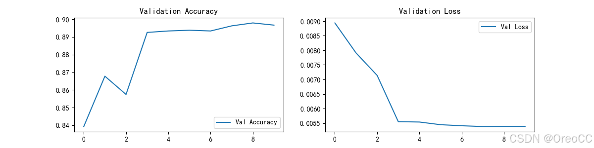
从结果图可以看出，整体效果起伏略大。

2. 调整学习率即优化器

将优化器调整为Adam，学习率调整至0.001，再次运行，结果如下：

| epoch: 1 |   50/ 152 batches| train_acc: 0.653 train_loss: 0.01796
| epoch: 1 |  100/ 152 batches| train_acc: 0.822 train_loss: 0.00886
| epoch: 1 |  150/ 152 batches| train_acc: 0.853 train_loss: 0.00729
---------------------------------------------------------------------
| epoch: 1 | time: 1.19s |valid_acc: 0.877 valid_loss: 0.006 | lr: 0.001000
---------------------------------------------------------------------
| epoch: 2 |   50/ 152 batches| train_acc: 0.859 train_loss: 0.00696
| epoch: 2 |  100/ 152 batches| train_acc: 0.866 train_loss: 0.00660
| epoch: 2 |  150/ 152 batches| train_acc: 0.877 train_loss: 0.00589
---------------------------------------------------------------------
| epoch: 2 | time: 1.05s |valid_acc: 0.882 valid_loss: 0.006 | lr: 0.001000
---------------------------------------------------------------------
| epoch: 3 |   50/ 152 batches| train_acc: 0.882 train_loss: 0.00586
| epoch: 3 |  100/ 152 batches| train_acc: 0.888 train_loss: 0.00574
| epoch: 3 |  150/ 152 batches| train_acc: 0.879 train_loss: 0.00580
---------------------------------------------------------------------
| epoch: 3 | time: 1.05s |valid_acc: 0.886 valid_loss: 0.006 | lr: 0.001000
---------------------------------------------------------------------
| epoch: 4 |   50/ 152 batches| train_acc: 0.881 train_loss: 0.00571
| epoch: 4 |  100/ 152 batches| train_acc: 0.893 train_loss: 0.00537
| epoch: 4 |  150/ 152 batches| train_acc: 0.891 train_loss: 0.00527
---------------------------------------------------------------------
| epoch: 4 | time: 1.06s |valid_acc: 0.892 valid_loss: 0.005 | lr: 0.001000
---------------------------------------------------------------------
| epoch: 5 |   50/ 152 batches| train_acc: 0.900 train_loss: 0.00479
| epoch: 5 |  100/ 152 batches| train_acc: 0.885 train_loss: 0.00534
| epoch: 5 |  150/ 152 batches| train_acc: 0.892 train_loss: 0.00534
---------------------------------------------------------------------
| epoch: 5 | time: 1.05s |valid_acc: 0.893 valid_loss: 0.005 | lr: 0.001000
---------------------------------------------------------------------
| epoch: 6 |   50/ 152 batches| train_acc: 0.900 train_loss: 0.00491
| epoch: 6 |  100/ 152 batches| train_acc: 0.896 train_loss: 0.00495
| epoch: 6 |  150/ 152 batches| train_acc: 0.902 train_loss: 0.00466
---------------------------------------------------------------------
| epoch: 6 | time: 1.05s |valid_acc: 0.892 valid_loss: 0.005 | lr: 0.001000
---------------------------------------------------------------------
| epoch: 7 |   50/ 152 batches| train_acc: 0.908 train_loss: 0.00442
| epoch: 7 |  100/ 152 batches| train_acc: 0.907 train_loss: 0.00435
| epoch: 7 |  150/ 152 batches| train_acc: 0.906 train_loss: 0.00437
---------------------------------------------------------------------
| epoch: 7 | time: 1.08s |valid_acc: 0.899 valid_loss: 0.005 | lr: 0.000100
---------------------------------------------------------------------
| epoch: 8 |   50/ 152 batches| train_acc: 0.915 train_loss: 0.00437
| epoch: 8 |  100/ 152 batches| train_acc: 0.904 train_loss: 0.00451
| epoch: 8 |  150/ 152 batches| train_acc: 0.912 train_loss: 0.00409
---------------------------------------------------------------------
| epoch: 8 | time: 1.16s |valid_acc: 0.901 valid_loss: 0.005 | lr: 0.000100
---------------------------------------------------------------------
| epoch: 9 |   50/ 152 batches| train_acc: 0.915 train_loss: 0.00396
| epoch: 9 |  100/ 152 batches| train_acc: 0.911 train_loss: 0.00426
| epoch: 9 |  150/ 152 batches| train_acc: 0.904 train_loss: 0.00453
---------------------------------------------------------------------
| epoch: 9 | time: 1.15s |valid_acc: 0.899 valid_loss: 0.005 | lr: 0.000100
---------------------------------------------------------------------
| epoch: 10 |   50/ 152 batches| train_acc: 0.914 train_loss: 0.00420
| epoch: 10 |  100/ 152 batches| train_acc: 0.912 train_loss: 0.00406
| epoch: 10 |  150/ 152 batches| train_acc: 0.912 train_loss: 0.00423
---------------------------------------------------------------------
| epoch: 10 | time: 1.17s |valid_acc: 0.900 valid_loss: 0.005 | lr: 0.000010
---------------------------------------------------------------------

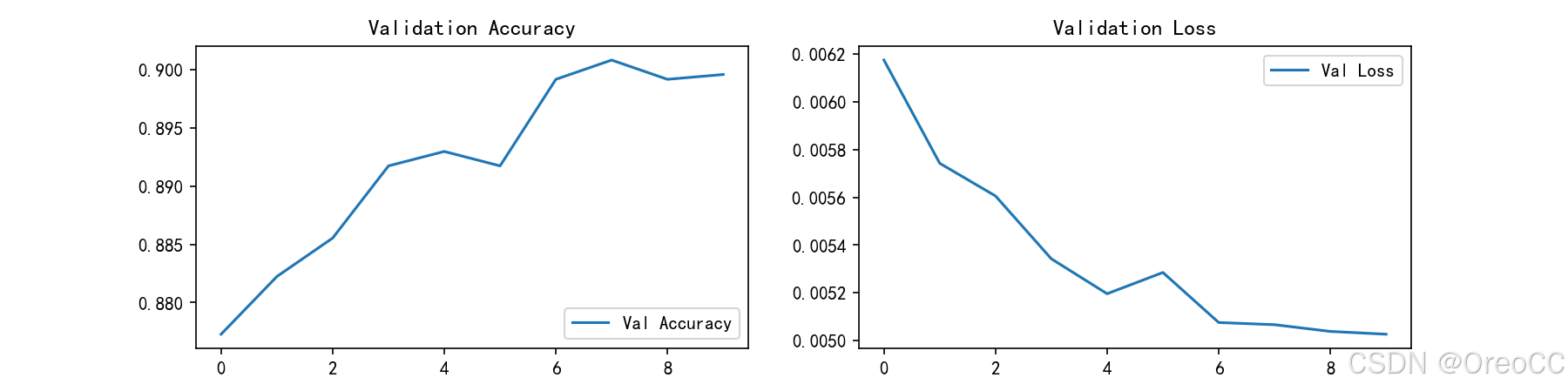
从结果图来看，此结果较为满意，准确率已提升至90%。 

3. 思考 

对使用Word2vec实现文本分类更加理解。面对海量数据时，应该考虑前期对数据进行预处理，去除停用词并进行清洗，同时可以考虑加深模型层次，尝试使用Transformer进行处理。