类 workbooks 的 open 方法无效_使用python+sklearn实现基于外存的文本分类方法
本示例展示了scikit-learn如何使用基于外存的方法来进行文本分类,即如何从无法放入主内存的数据中进行机器学习。我们使用一个在线分类器,即一个支持partial_fit 方法的分类器,该分类器将提供一批示例。为了保证特征空间在一段时间内保持不变,我们使用了一个HashingVectorizer,它将每个示例投影到同一个特征空间中,这在文本分类中是非常有用的,因为每个batch中可能...
·
本示例展示了scikit-learn如何使用基于外存的方法来进行文本分类,即如何从无法放入主内存的数据中进行机器学习。我们使用一个在线分类器,即一个支持partial_fit 方法的分类器,该分类器将提供一批示例。为了保证特征空间在一段时间内保持不变,我们使用了一个HashingVectorizer,它将每个示例投影到同一个特征空间中,这在文本分类中是非常有用的,因为每个batch中可能会出现新的特征(单词)。
# 作者: Eustache Diemert #          @FedericoV # 许可证: BSD 3 clause
from glob import glob
import itertools
import os.path
import re
import tarfile
import time
import sys
import numpy as np
import matplotlib.pyplot as plt
from matplotlib import rcParams
from html.parser import HTMLParser
from urllib.request import urlretrieve
from sklearn.datasets import get_data_home
from sklearn.feature_extraction.text import HashingVectorizer
from sklearn.linear_model import SGDClassifier
from sklearn.linear_model import PassiveAggressiveClassifier
from sklearn.linear_model import Perceptron
from sklearn.naive_bayes import MultinomialNB
def _not_in_sphinx():# Hack to detect whether we are running by the sphinx builderreturn '__file__' in globals()
Reuters 数据集相关例程
本示例中使用的数据集是UCI ML存储库提供的Reuters-21578,它会在首次运行时自动下载并解压缩。class ReutersParser(HTMLParser):"""实用程序类,用于解析SGML文件并一次生成一个文档。"""
def __init__(self, encoding='latin-1'):
HTMLParser.__init__(self)
self._reset()
self.encoding = encoding
def handle_starttag(self, tag, attrs):
method = 'start_' + tag
getattr(self, method, lambda x: None)(attrs)
def handle_endtag(self, tag):
method = 'end_' + tag
getattr(self, method, lambda: None)()
def _reset(self):
self.in_title = 0
self.in_body = 0
self.in_topics = 0
self.in_topic_d = 0
self.title = ""
self.body = ""
self.topics = []
self.topic_d = ""
def parse(self, fd):
self.docs = []for chunk in fd:
self.feed(chunk.decode(self.encoding))for doc in self.docs:
yield doc
self.docs = []
self.close()
def handle_data(self, data):if self.in_body:
self.body += dataelif self.in_title:
self.title += dataelif self.in_topic_d:
self.topic_d += data
def start_reuters(self, attributes):
pass
def end_reuters(self):
self.body = re.sub(r'\s+', r' ', self.body)
self.docs.append({'title': self.title,'body': self.body,'topics': self.topics})
self._reset()
def start_title(self, attributes):
self.in_title = 1
def end_title(self):
self.in_title = 0
def start_body(self, attributes):
self.in_body = 1
def end_body(self):
self.in_body = 0
def start_topics(self, attributes):
self.in_topics = 1
def end_topics(self):
self.in_topics = 0
def start_d(self, attributes):
self.in_topic_d = 1
def end_d(self):
self.in_topic_d = 0
self.topics.append(self.topic_d)
self.topic_d = ""
def stream_reuters_documents(data_path=None):"""遍历Reuters数据集的文档。
如果`data_path`目录不存在,Reuters文件将自动下载并解压缩,文档将表示
成键(key)为'body' (str), 'title' (str), 'topics' (list(str))的字典。
"""
DOWNLOAD_URL = ('http://archive.ics.uci.edu/ml/machine-learning-databases/''reuters21578-mld/reuters21578.tar.gz')
ARCHIVE_FILENAME = 'reuters21578.tar.gz'if data_path is None:
data_path = os.path.join(get_data_home(), "reuters")if not os.path.exists(data_path):"""Download the dataset."""print("downloading dataset (once and for all) into %s" %
data_path)
os.mkdir(data_path)
def progress(blocknum, bs, size):
total_sz_mb = '%.2f MB' % (size / 1e6)
current_sz_mb = '%.2f MB' % ((blocknum * bs) / 1e6)if _not_in_sphinx():
sys.stdout.write('\rdownloaded %s / %s' % (current_sz_mb, total_sz_mb))
archive_path = os.path.join(data_path, ARCHIVE_FILENAME)
urlretrieve(DOWNLOAD_URL, filename=archive_path,
reporthook=progress)if _not_in_sphinx():
sys.stdout.write('\r')print("untarring Reuters dataset...")
tarfile.open(archive_path, 'r:gz').extractall(data_path)print("done.")
parser = ReutersParser()for filename in glob(os.path.join(data_path, "*.sgm")):for doc in parser.parse(open(filename, 'rb')):
yield doc主程序
创建矢量化器(vectorizer)并将特征数量限制为合理的最大值。vectorizer = HashingVectorizer(decode_error='ignore', n_features=2 ** 18,
alternate_sign=False)# 在解析的Reuters SGML文件上进行迭代。
data_stream = stream_reuters_documents()# 我们学习了"acq"类和所有其他类之间的二分类。# 选择"acq",是因为它或多或少地均匀地分布在路透社的文件中。# 对于其他数据集,应该创建一个测试集,其中包含一部分真实的正实例。
all_classes = np.array([0, 1])
positive_class = 'acq'# 下面是一些支持`partial_fit`方法的分类器
partial_fit_classifiers = {'SGD': SGDClassifier(max_iter=5),'Perceptron': Perceptron(),'NB Multinomial': MultinomialNB(alpha=0.01),'Passive-Aggressive': PassiveAggressiveClassifier(),
}
def get_minibatch(doc_iter, size, pos_class=positive_class):"""提取一小批示例,返回一个元组 X_text,y。
注意: size 在排除未分配主题的无效文档之前的。
"""
data = [('{title}\n\n{body}'.format(**doc), pos_class in doc['topics'])for doc in itertools.islice(doc_iter, size)if doc['topics']]if not len(data):return np.asarray([], dtype=int), np.asarray([], dtype=int)
X_text, y = zip(*data)return X_text, np.asarray(y, dtype=int)
def iter_minibatches(doc_iter, minibatch_size):"""小批量的生成器。"""
X_text, y = get_minibatch(doc_iter, minibatch_size)while len(X_text):
yield X_text, y
X_text, y = get_minibatch(doc_iter, minibatch_size)# 测试数据统计
test_stats = {'n_test': 0, 'n_test_pos': 0}# 首先我们举了一些例子来估计准确度
n_test_documents = 1000
tick = time.time()
X_test_text, y_test = get_minibatch(data_stream, 1000)
parsing_time = time.time() - tick
tick = time.time()
X_test = vectorizer.transform(X_test_text)
vectorizing_time = time.time() - tick
test_stats['n_test'] += len(y_test)
test_stats['n_test_pos'] += sum(y_test)print("Test set is %d documents (%d positive)" % (len(y_test), sum(y_test)))
def progress(cls_name, stats):"""报告进度信息,返回一个字符串。"""
duration = time.time() - stats['t0']
s = "%20s classifier : \t" % cls_name
s += "%(n_train)6d train docs (%(n_train_pos)6d positive) " % stats
s += "%(n_test)6d test docs (%(n_test_pos)6d positive) " % test_stats
s += "accuracy: %(accuracy).3f " % stats
s += "in %.2fs (%5d docs/s)" % (duration, stats['n_train'] / duration)return s
cls_stats = {}for cls_name in partial_fit_classifiers:
stats = {'n_train': 0, 'n_train_pos': 0,'accuracy': 0.0, 'accuracy_history': [(0, 0)], 't0': time.time(),'runtime_history': [(0, 0)], 'total_fit_time': 0.0}
cls_stats[cls_name] = stats
get_minibatch(data_stream, n_test_documents)# 丢弃测试集# 我们将为分类器提供1000(mini-batches=1000)个文档;# 这意味着在任何时候最多有1000个文档在内存中。# 文档的batch越小,部分拟合方法的相对开销越大。
minibatch_size = 1000# 创建解析Reuters SGML文件并作为流在文档上迭代的 data_stream 。
minibatch_iterators = iter_minibatches(data_stream, minibatch_size)
total_vect_time = 0.0# 主循环:迭代mini-batches个示例for i, (X_train_text, y_train) in enumerate(minibatch_iterators):
tick = time.time()
X_train = vectorizer.transform(X_train_text)
total_vect_time += time.time() - tickfor cls_name, cls in partial_fit_classifiers.items():
tick = time.time()# 用当前小批量中的实例更新估计器
cls.partial_fit(X_train, y_train, classes=all_classes)# 累积测试准确度统计信息
cls_stats[cls_name]['total_fit_time'] += time.time() - tick
cls_stats[cls_name]['n_train'] += X_train.shape[0]
cls_stats[cls_name]['n_train_pos'] += sum(y_train)
tick = time.time()
cls_stats[cls_name]['accuracy'] = cls.score(X_test, y_test)
cls_stats[cls_name]['prediction_time'] = time.time() - tick
acc_history = (cls_stats[cls_name]['accuracy'],
cls_stats[cls_name]['n_train'])
cls_stats[cls_name]['accuracy_history'].append(acc_history)
run_history = (cls_stats[cls_name]['accuracy'],
total_vect_time + cls_stats[cls_name]['total_fit_time'])
cls_stats[cls_name]['runtime_history'].append(run_history)if i % 3 == 0:print(progress(cls_name, cls_stats[cls_name]))if i % 3 == 0:print('\n')Test set is 973 documents (125 positive)
SGD classifier : 965 train docs ( 134 positive) 973 test docs ( 125 positive) accuracy: 0.921 in 0.68s ( 1419 docs/s)
Perceptron classifier : 965 train docs ( 134 positive) 973 test docs ( 125 positive) accuracy: 0.872 in 0.69s ( 1407 docs/s)
NB Multinomial classifier : 965 train docs ( 134 positive) 973 test docs ( 125 positive) accuracy: 0.874 in 0.71s ( 1355 docs/s)
Passive-Aggressive classifier : 965 train docs ( 134 positive) 973 test docs ( 125 positive) accuracy: 0.920 in 0.71s ( 1350 docs/s)
SGD classifier : 3790 train docs ( 506 positive) 973 test docs ( 125 positive) accuracy: 0.963 in 1.96s ( 1932 docs/s)
Perceptron classifier : 3790 train docs ( 506 positive) 973 test docs ( 125 positive) accuracy: 0.949 in 1.96s ( 1929 docs/s)
NB Multinomial classifier : 3790 train docs ( 506 positive) 973 test docs ( 125 positive) accuracy: 0.884 in 1.98s ( 1912 docs/s)
Passive-Aggressive classifier : 3790 train docs ( 506 positive) 973 test docs ( 125 positive) accuracy: 0.947 in 1.98s ( 1910 docs/s)
SGD classifier : 6523 train docs ( 916 positive) 973 test docs ( 125 positive) accuracy: 0.950 in 3.21s ( 2031 docs/s)
Perceptron classifier : 6523 train docs ( 916 positive) 973 test docs ( 125 positive) accuracy: 0.923 in 3.21s ( 2030 docs/s)
NB Multinomial classifier : 6523 train docs ( 916 positive) 973 test docs ( 125 positive) accuracy: 0.909 in 3.23s ( 2019 docs/s)
Passive-Aggressive classifier : 6523 train docs ( 916 positive) 973 test docs ( 125 positive) accuracy: 0.953 in 3.23s ( 2017 docs/s)
SGD classifier : 9434 train docs ( 1242 positive) 973 test docs ( 125 positive) accuracy: 0.927 in 4.48s ( 2107 docs/s)
Perceptron classifier : 9434 train docs ( 1242 positive) 973 test docs ( 125 positive) accuracy: 0.947 in 4.48s ( 2106 docs/s)
NB Multinomial classifier : 9434 train docs ( 1242 positive) 973 test docs ( 125 positive) accuracy: 0.918 in 4.50s ( 2098 docs/s)
Passive-Aggressive classifier : 9434 train docs ( 1242 positive) 973 test docs ( 125 positive) accuracy: 0.956 in 4.50s ( 2096 docs/s)
SGD classifier : 11845 train docs ( 1468 positive) 973 test docs ( 125 positive) accuracy: 0.949 in 5.75s ( 2061 docs/s)
Perceptron classifier : 11845 train docs ( 1468 positive) 973 test docs ( 125 positive) accuracy: 0.942 in 5.75s ( 2060 docs/s)
NB Multinomial classifier : 11845 train docs ( 1468 positive) 973 test docs ( 125 positive) accuracy: 0.922 in 5.77s ( 2054 docs/s)
Passive-Aggressive classifier : 11845 train docs ( 1468 positive) 973 test docs ( 125 positive) accuracy: 0.942 in 5.77s ( 2053 docs/s)
SGD classifier : 14770 train docs ( 1856 positive) 973 test docs ( 125 positive) accuracy: 0.959 in 7.10s ( 2079 docs/s)
Perceptron classifier : 14770 train docs ( 1856 positive) 973 test docs ( 125 positive) accuracy: 0.956 in 7.11s ( 2078 docs/s)
NB Multinomial classifier : 14770 train docs ( 1856 positive) 973 test docs ( 125 positive) accuracy: 0.925 in 7.12s ( 2073 docs/s)
Passive-Aggressive classifier : 14770 train docs ( 1856 positive) 973 test docs ( 125 positive) accuracy: 0.957 in 7.13s ( 2072 docs/s)
SGD classifier : 17723 train docs ( 2218 positive) 973 test docs ( 125 positive) accuracy: 0.959 in 8.47s ( 2093 docs/s)
Perceptron classifier : 17723 train docs ( 2218 positive) 973 test docs ( 125 positive) accuracy: 0.938 in 8.47s ( 2092 docs/s)
NB Multinomial classifier : 17723 train docs ( 2218 positive) 973 test docs ( 125 positive) accuracy: 0.925 in 8.49s ( 2087 docs/s)
Passive-Aggressive classifier : 17723 train docs ( 2218 positive) 973 test docs ( 125 positive) accuracy: 0.962 in 8.49s ( 2087 docs/s)绘制结果
该图代表了分类器的学习曲线:分类精度在小批量过程中的变化。在前1000个样本中测量准确度,并将其作为验证集。为了限制内存消耗,在将示例输入给学习器之前,将其排成固定数量的队列。def plot_accuracy(x, y, x_legend):"""绘图准确度"""
x = np.array(x)
y = np.array(y)
plt.title('Classification accuracy as a function of %s' % x_legend)
plt.xlabel('%s' % x_legend)
plt.ylabel('Accuracy')
plt.grid(True)
plt.plot(x, y)
rcParams['legend.fontsize'] = 10
cls_names = list(sorted(cls_stats.keys()))# 绘制准确度的变化
plt.figure()for _, stats in sorted(cls_stats.items()):# Plot accuracy evolution with #examples
accuracy, n_examples = zip(*stats['accuracy_history'])
plot_accuracy(n_examples, accuracy, "training examples (#)")
ax = plt.gca()
ax.set_ylim((0.8, 1))
plt.legend(cls_names, loc='best')
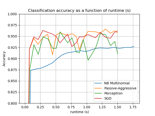
plt.figure()for _, stats in sorted(cls_stats.items()):# Plot accuracy evolution with runtime
accuracy, runtime = zip(*stats['runtime_history'])
plot_accuracy(runtime, accuracy, 'runtime (s)')
ax = plt.gca()
ax.set_ylim((0.8, 1))
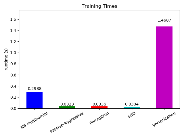
plt.legend(cls_names, loc='best')# 绘制拟合时间
plt.figure()
fig = plt.gcf()
cls_runtime = [stats['total_fit_time']for cls_name, stats in sorted(cls_stats.items())]
cls_runtime.append(total_vect_time)
cls_names.append('Vectorization')
bar_colors = ['b', 'g', 'r', 'c', 'm', 'y']
ax = plt.subplot(111)
rectangles = plt.bar(range(len(cls_names)), cls_runtime, width=0.5,
color=bar_colors)
ax.set_xticks(np.linspace(0, len(cls_names) - 1, len(cls_names)))
ax.set_xticklabels(cls_names, fontsize=10)
ymax = max(cls_runtime) * 1.2
ax.set_ylim((0, ymax))
ax.set_ylabel('runtime (s)')
ax.set_title('Training Times')
def autolabel(rectangles):"""在矩形上附加一些文本vi自动标签"""for rect in rectangles:
height = rect.get_height()
ax.text(rect.get_x() + rect.get_width() / 2.,
1.05 * height, '%.4f' % height,
ha='center', va='bottom')
plt.setp(plt.xticks()[1], rotation=30)
autolabel(rectangles)
plt.tight_layout()
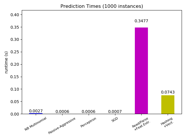
plt.show()# 绘制预测时间
plt.figure()
cls_runtime = []
cls_names = list(sorted(cls_stats.keys()))for cls_name, stats in sorted(cls_stats.items()):
cls_runtime.append(stats['prediction_time'])
cls_runtime.append(parsing_time)
cls_names.append('Read/Parse\n+Feat.Extr.')
cls_runtime.append(vectorizing_time)
cls_names.append('Hashing\n+Vect.')
ax = plt.subplot(111)
rectangles = plt.bar(range(len(cls_names)), cls_runtime, width=0.5,
color=bar_colors)
ax.set_xticks(np.linspace(0, len(cls_names) - 1, len(cls_names)))
ax.set_xticklabels(cls_names, fontsize=8)
plt.setp(plt.xticks()[1], rotation=30)
ymax = max(cls_runtime) * 1.2
ax.set_ylim((0, ymax))
ax.set_ylabel('runtime (s)')
ax.set_title('Prediction Times (%d instances)' % n_test_documents)
autolabel(rectangles)
plt.tight_layout()
plt.show()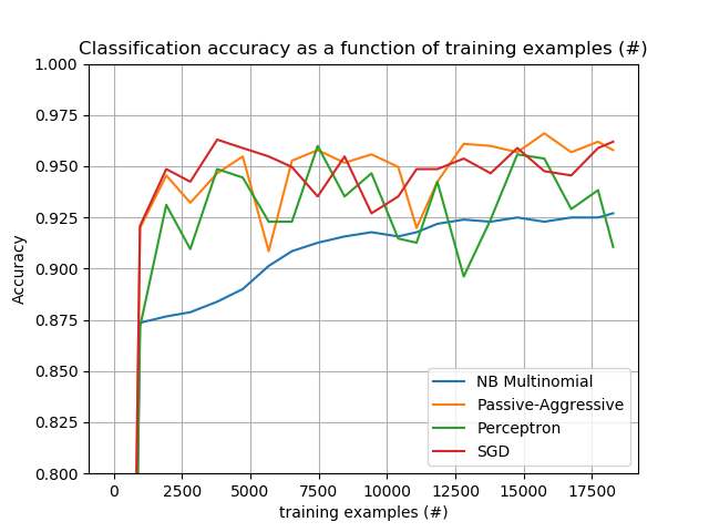

下载python源代码:plot_out_of_core_classification.py下载Jupyter notebook源代码:plot_out_of_core_classification.ipynb由Sphinx-Gallery生成的画廊 ☆☆☆为方便大家查阅,小编已将scikit-learn学习路线专栏文章统一整理到公众号底部菜单栏,同步更新中,关注公众号,点击左下方“系列文章”,如图:
 欢迎大家和我一起沿着scikit-learn文档这条路线,一起巩固机器学习算法基础。(添加微信:mthler,备注:sklearn学习,一起进【sklearn机器学习进步群】开启打怪升级的学习之旅。)

魔乐社区(Modelers.cn) 是一个中立、公益的人工智能社区,提供人工智能工具、模型、数据的托管、展示与应用协同服务,为人工智能开发及爱好者搭建开放的学习交流平台。社区通过理事会方式运作,由全产业链共同建设、共同运营、共同享有,推动国产AI生态繁荣发展。
更多推荐


 0
0 0
0- 0


 已为社区贡献5条内容

所有评论(0)