一、模型介绍

论文为《TabNet: Attentive Interpretable Tabular Learning》发表于2021年，属于Google Cloud AI。该研究针对表格数据提出了一种新的深度神经网络（DNN）架构TabNet，旨在解决传统深度学习在表格数据上表现不如决策树模型的问题，同时提升性能和可解释性。

TabNet模型融合了多种先进思想：它将Transformer的注意力机制（赋予模型动态、稀疏地“聚焦”于最重要特征的能力）、Boosting的序列化决策思想（分步、迭代地做出决策）以及自监督学习的表示学习能力（在正式训练前，让模型预先学习特征间的内在关系，为后续的智能决策提供“先验知识）巧妙地结合在了一起，用于解决表格数据问题。

保留DNN的end-to-end和representation learning特点的基础上，还拥有了树模型的可解释性和稀疏特征选择的优点

TabNet 的工作方式（通俗的方式理解模型）

Boosting的序列化决策思想（比如GBDT 通过拟合上一步的预测残差不断训练迭代模型）

• 使用一部分特征（通过自监督学习+注意力选择），做出一个初步的预测贡献。

• TabNet不像Boosting那样显式地计算一个 y_true - y_pred 的残差，它通过特征选择机制达到了类似的效果。当第二步的注意力模块被告知“这些特征已经被用过了”时，它实际上是在被引导去关注那些在第一步中未能充分解释目标变量方差的特征。这可以被看作是在特征空间中的“残差学习”。

• 基于新选出的特征，产生一个新的“预测贡献”。这个贡献的作用就是修正或细化第一步的判断。

• 这个过程在多个步骤中重复，每一步都试图利用新的特征组合来进一步完善整体的预测。

TabNet架构设计

TabNet 将预测分解为多个步骤。在每一步，它都用一个注意力模块（Attentive Transformer）来智能地、稀疏地挑选出一组当前最相关的特征，然后用另一个模块（Feature Transformer）来处理这些特征并得出初步结论。这个过程是序列化的，因为后一步的选择会受到前一步的影响，从而使模型能够全面而高效地利用所有特征信息，最终做出高质量的预测。

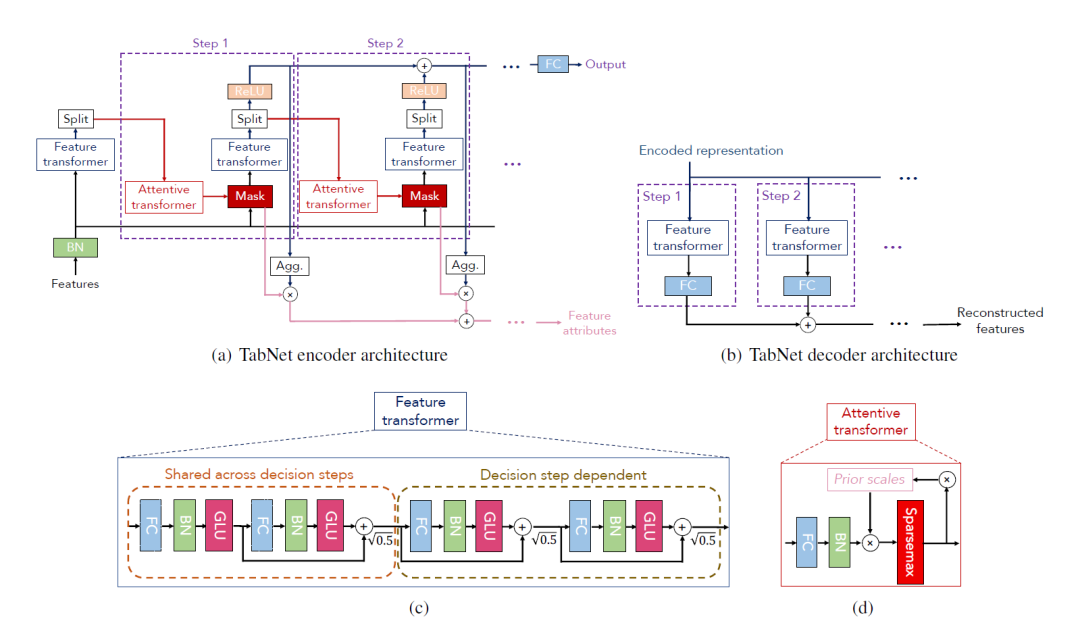
自监督学习

在整个有监督的决策流程开始之前，TabNet可以通过一个自监督的预训练任务来“热身”。模型通过随机遮蔽（Mask）一部分特征，然后尝试用剩余的特征来预测被遮蔽的内容。

• 赋予模型关于“特征关系图谱”的先验知识：模型被迫学习到特征之间复杂的相关、互补或冗余关系。

• 提升决策效率：当进入正式的序列化决策流程时，Attentive Transformer不再是盲目选择特征，而是基于已经学到的“常识”，做出更明智、更高效的特征选择。

  
  

Attentive Transformer (注意力转换器)

Attentive Transformer是决策的起点，它的核心使命是回答：“在当前步骤，我应该关注哪些特征？”

它接收上一步处理过的信息，利用注意力机制为所有特征计算出一个“特征权重”。特征权重基于sparsemax的激活函数和正则化，使得注意力模块每次只选择少数几个最关键的特征，将其权重设为非零，而其他大量无关特征的权重则为零，从而完成动态选择最重要特征的目的。

序列化更新：它有一个“记忆机制”。在生成新的Mask时，它会参考一个“先验尺度”（Prior Scale），该尺度记录了每个特征在之前所有步骤中被使用的总程度。如果一个特征已被频繁使用，模型会被激励去降低对它的关注，转而探索新的、未被充分利用的特征。

Feature Transformer (特征转换器)

一旦Attentive Transformer选定了特征，Feature Transformer就接手处理，它的使命是：“利用这些选中的特征，我能得出什么结论？”

该模块接收 Attention Mask M_i 筛选和加权后的特征，通过几层神经网络对被选中的特征进行复杂的非线性变换，提取出有用的信息，并为最终预测贡献一部分结果。

多步骤决策

所有决策步骤（比如N步）都完成后，模型会将每个步骤产生的“预测贡献”加权求和，得到最终的预测结果。

其中，加权系数与每个步骤探索“新特征”的程度有关，具体来说，与(1 - Prior_i)有关（Prior_i是到第i步为止的特征累积使用度）。这种机制确保了最终的预测结果是建立在一系列互补、多样化的特征视角之上，从而更加鲁棒和准确。

---

二、代码实现

Pytorch-tabnet可以实现以下任务：

• TabNetClassifier：二元分类和多类分类问题
• TabNetRegressor：简单和多任务回归问题
• TabNetMultiTaskClassifier：多任务多分类问题

整个模型可分为自监督预训练 (Self-supervised Pre-training)+有监督微调 (Supervised Fine-tuning)，官方展示的二分类或多分类示例中仅仅展示了有监督微调部分。下面代码展示页只包括模型训练部分：

Step1：包和数据载入预处理

from pytorch_tabnet.tab_model import TabNetClassifier

import torch
from sklearn.preprocessing import LabelEncoder
from sklearn.metrics import roc_auc_score

import pandas as pd
import numpy as np
np.random.seed(0)

import scipy

import wget
from pathlib import Path

from matplotlib import pyplot as plt
# %matplotlib inline

import os
os.environ['CUDA_VISIBLE_DEVICES'] = f"0"
import torch
torch.__version__
import optuna
import scipy.sparse

# filein_name = filein.replace(".csv","")
filein_name ="tmp"
save_path = './Result_' + filein_name + '_s73_try1/'  # raw_dataset

paths = [save_path + "/input/", save_path + "/result/", save_path + "/models/"]
for path in paths:
    if not os.path.exists(path):
        os.makedirs(path)

# 数据加载
url = "https://archive.ics.uci.edu/ml/machine-learning-databases/adult/adult.data"
dataset_name = 'census-income'
out = Path(os.getcwd()+'/data/'+dataset_name+'.csv')
out.parent.mkdir(parents=True, exist_ok=True)
if out.exists():
    print("File already exists.")
else:
    print("Downloading file...")
    wget.download(url, out.as_posix())
train = pd.read_csv(out)
target = ' <=50K'

# 数据预处理，比如标签编码 
nunique = train.nunique()
types = train.dtypes

categorical_columns = []
categorical_dims =  {}
for col in train.columns:
    if types[col] == 'object' or nunique[col] < 200:
        print(col, train[col].nunique())
        l_enc = LabelEncoder()
        train[col] = train[col].fillna("Unknown")
        train[col] = l_enc.fit_transform(train[col].values)
        categorical_columns.append(col)
        categorical_dims[col] = len(l_enc.classes_)
#     else:
#         train.fillna(train.loc[train_indices, col].mean(), inplace=True)

# 划分数据集
if "Set" not in train.columns:
    train["Set"] = np.random.choice(["train", "valid", "test"], p =[.8, .1, .1], size=(train.shape[0],))
print(train["Set"].value_counts())

train_indices = train[train.Set=="train"].index
valid_indices = train[train.Set=="valid"].index
test_indices = train[train.Set=="test"].index

# 生成cat_idxs，cat_dims等参数
unused_feat = ['Set']

features = [ col for col in train.columns if col not in unused_feat+[target]] 

cat_idxs = [ i for i, f in enumerate(features) if f in categorical_columns]

cat_dims = [ categorical_dims[f] for i, f in enumerate(features) if f in categorical_columns]

grouped_features = [[0, 1, 2], [8, 9, 10]]

X_train = train[features].values[train_indices]
y_train = train[target].values[train_indices]

X_valid = train[features].values[valid_indices]
y_valid = train[target].values[valid_indices]

X_test = train[features].values[test_indices]
y_test = train[target].values[test_indices]

Step2： 模型训练

Step 2.0：参数解释

数据处理方面

• cat_idxs： 所有类别特征在输入特征矩阵 X 中的列索引
• cat_dims：含了每个类别特征的基数（cardinality），也就是该特征有多少个不同的取值。
• cat_emb_dim：将类别变量中的每一个类别表示成一个长度为多长的特征。
• grouped_features：比如独热编码后的特征，比如身高体重与BMI

模型训练参数：

• n_d, n_a:代表决策流（decision stream）和注意力流（attention stream）的输出维度。它们共同决定了模型每一步的“宽度”。通常将它们设置为相等的值，例如 8, 16, 32, 64。从较小的值开始（如 n_d=8, n_a=8），如果模型欠拟合（训练集和验证集表现都不好），则逐步增大。如果模型过拟合（训练集表现远好于验证集），可以尝试减小它们或增加正则化。
• n_steps：模型中决策步骤的数量。每个步骤都会选择一部分特征进行处理。值越大，模型越复杂，理论上能学习更复杂的模式。通常取值在 3 到 10 之间。更多的步骤会增加训练时间，也可能导致过拟合。
• gamma:特征重用系数。值越大（接近2.0），每个特征在所有决策步骤中被使用的可能性就越小，鼓励模型在不同步骤关注不同特征。值越小（接近1.0），特征可以被更频繁地重用。如果感觉模型在不同步骤总是关注相同的特征，可以适当增大 gamma。
• lambda_sparse:稀疏性正则化系数。这是TabNet的一个关键特性，它鼓励模型在每一步只选择最重要的少数特征，从而实现可解释性并防止过拟合。值越大，特征选择越稀疏。如果模型严重过拟合，可以尝试增大此值。如果模型欠拟合，或者你发现重要特征没有被选入，可以减小此值。搜索范围建议: [1e-4, 1e-3, 1e-2, 0.1] (通常在对数尺度上搜索)

处理数据类别不平衡（SMOTE和weights通常只用一种）

• weights: 设置类别权重，也是处理不平衡数据的方法。weights=1 表示所有类别权重相同。如果你有类别不平衡问题，可以设置为 0（自动计算权重，使得少数类有更高权重）

优化器与学习率调度器调优

• optimizer_fn: Adam 通常是个不错的选择。AdamW 是 Adam 的改进版，可以尝试替换。在对数尺度上搜索，通常 1e-3 到 2e-2 是一个比较常见的范围。
• scheduler_fn 和 scheduler_params: ReduceLROnPlateau 通常是更好的选择。它会监测验证集上的指标（如 valid_auc），当指标在一定 patience 内不再提升时，自动降低学习率。

Step 2.1： 基于optuna自动搜索超参数

import optuna
import torch
import scipy.sparse
max_epochs = 50 if not os.getenv("CI", False) else 2

# 数据增强
from pytorch_tabnet.augmentations import ClassificationSMOTE
#aug = ClassificationSMOTE(p=0.2)

# 此时X_train, y_train, X_valid, y_valid, cat_idxs, cat_dims, grouped_features 已定义

def objective(trial):
    # 定义要搜索的超参数空间
    n_d = trial.suggest_int("n_d", 8, 32, step=8) 
    n_steps = trial.suggest_int("n_steps", 3, 7) # 决策步骤数
    gamma = trial.suggest_float("gamma", 1.0, 2.0)# 特征重用系数，值越大，特征重用可能性越小
    lambda_sparse = trial.suggest_float("lambda_sparse", 1e-4, 1e-2, log=True) # 值越大，特征选择越稀疏；过拟合，增大此值，使模型更专注，减少对噪音的学习
    
    lr = trial.suggest_float("lr", 1e-3, 3e-2, log=True)
    virtual_batch_size = trial.suggest_categorical("virtual_batch_size", [128, 256])
    weight_decay = trial.suggest_float("weight_decay", 1e-6, 1e-3, log=True)
    mask_type = trial.suggest_categorical("mask_type", ["entmax", "sparsemax"])
    
    aug_p = trial.suggest_float("aug_p", 0.1, 0.4, step=0.1)
    aug = ClassificationSMOTE(p=aug_p)
    
    
    # 设置模型参数
    tabnet_params = {
        "cat_idxs": cat_idxs,
        "cat_dims": cat_dims,
        "cat_emb_dim": 2,
        "grouped_features": grouped_features,
        
        "n_d": n_d,
        "n_a": n_d,  # 保持 n_a 和 n_d 一致
        "n_steps": n_steps,
        "gamma": gamma,
        "lambda_sparse": lambda_sparse,
        "mask_type": mask_type, # sparsemax，entmax
        
        "optimizer_fn": torch.optim.AdamW,  
        "optimizer_params": dict(lr=lr, weight_decay=weight_decay),
        "scheduler_fn": torch.optim.lr_scheduler.ReduceLROnPlateau,
        "scheduler_params":dict(mode="max",patience=5, min_lr=1e-5,factor=0.5)
    }

    clf = TabNetClassifier(**tabnet_params)
    
    # 训练模型：在超参数搜索时，可以适当减少 max_epochs 和 patience 来加速
    max_epochs = 50
    patience = 10
    
    clf.fit(
        X_train=X_train, y_train=y_train,
        eval_set=[(X_valid, y_valid)],
        eval_name=['valid'],
        eval_metric=['auc'],
        max_epochs=max_epochs,
        patience=patience,
        batch_size=2048, # 增大 batch_size
        virtual_batch_size=virtual_batch_size,
        num_workers=0,
        drop_last=False, # 在搜索时可以先关掉
        augmentations=aug, # 暂时关闭增强，专注于模型结构
    )
    
    # 返回要优化的目标
    # clf.best_cost 是验证集上最好的损失，我们希望最大化AUC
    # clf.history['valid_auc'] 是一个列表，取最后一个值或最大值
    valid_auc = max(clf.history['valid_auc'])
    return valid_auc

# 开始优化
study = optuna.create_study(direction="maximize", study_name='TabNet optimization') # direction="maximize" 因为我们要最大化 AUC
study.pruners = optuna.pruners.MedianPruner() # 增加剪枝，提前终止不好的试验
study.optimize(objective, n_trials=2, timeout=6*60) # n_trials 是你想要尝试的超参数组合数量

# 输出最佳参数
print("Best trial:")
trial = study.best_trial
print("  Params: ")
for key, value in trial.params.items():
    print(f"    {key}: {value}")

best_params = trial.params

Step 2.2： 基于最优超参数训练模型

tabnet_params = dict(cat_idxs=cat_idxs,
                     cat_dims=cat_dims,
                     cat_emb_dim=2,
                     grouped_features=grouped_features,
                     
                     n_d=best_params['n_d'], n_a=best_params['n_d'], n_steps=best_params['n_steps'], gamma=best_params['gamma'],
                     lambda_sparse=best_params['lambda_sparse'],mask_type=best_params['mask_type'],
                     
                     optimizer_fn=torch.optim.Adam,
                     optimizer_params=dict(lr=best_params["lr"], weight_decay=best_params["weight_decay"]),
                     scheduler_fn=torch.optim.lr_scheduler.ReduceLROnPlateau,
                     scheduler_params=dict(mode="max",
                                           patience=5,
                                           min_lr=1e-5,
                                           factor=0.5),
                     verbose=0
                     )

clf = TabNetClassifier(**tabnet_params)

# This illustrates the behaviour of the model's fit method using Compressed Sparse Row matrices
sparse_X_train = scipy.sparse.csr_matrix(X_train)  # Create a CSR matrix from X_train 优化内存使用和加速模型训练。
sparse_X_valid = scipy.sparse.csr_matrix(X_valid)   
    
# Fitting the model
max_epochs = 50
aug = ClassificationSMOTE(p=best_params["aug_p"])
clf.fit(
    X_train=sparse_X_train, y_train=y_train,
    eval_set=[(sparse_X_train, y_train), (sparse_X_valid, y_valid)],
    eval_name=['train', 'valid'],
    eval_metric=['auc'],
    
    max_epochs=max_epochs, patience=20,
    batch_size=1024, virtual_batch_size=128,
    num_workers=0,
    drop_last=True, #丢弃最后一个批次
    
    # 类别不平衡
    weights=0,
    augmentations=aug,  
    
    compute_importance=True
)

# plot losses
plt.figure(figsize=(3,2))
plt.plot(clf.history['loss'])
plt.show()

# plot learning rates
plt.figure(figsize=(3,2))
plt.plot(clf.history['lr'])
plt.show()

# plot auc
plt.figure(figsize=(3,2))
plt.plot(clf.history['train_auc'], label='Train AUC')
plt.plot(clf.history['valid_auc'], label='Valid AUC')
plt.legend()
plt.show()

Step 2.3： 预测及结果保存

# save tabnet model
savefile = save_path + "/models/tabnet_model" 
saved_filepath = clf.save_model(savefile)

# load tabnet model
loaded_model = TabNetClassifier()
loaded_model.load_model(saved_filepath)
loaded_model

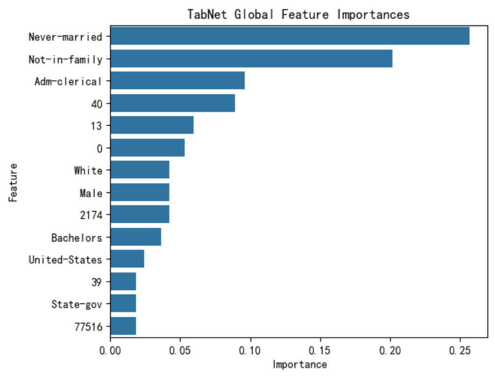
Step 3：特征可解释性-tabnet固有

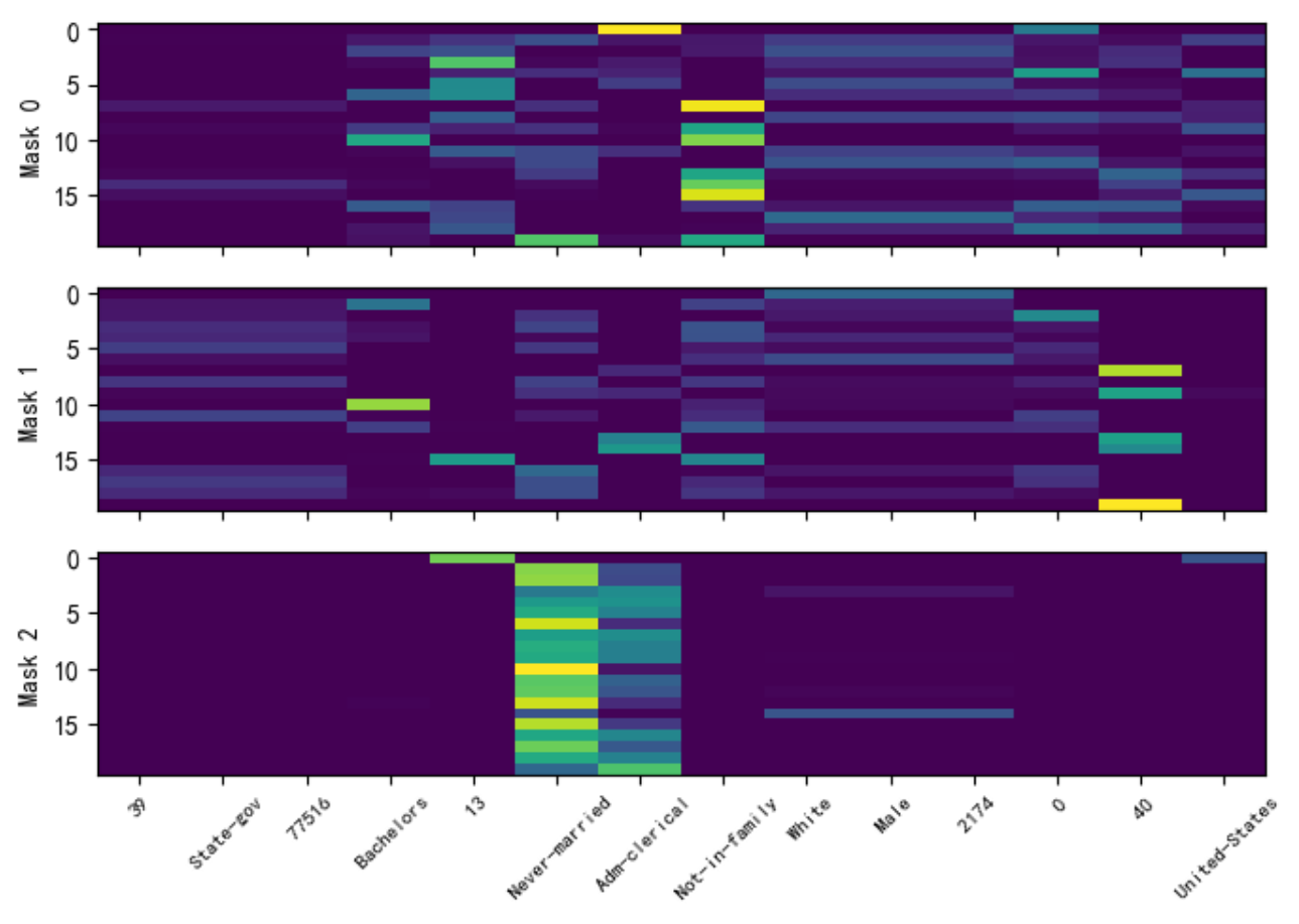
explain_matrix, masks = clf.explain(X_test) 
# explain_matrix 是对所有决策步骤 (steps) 的掩码 (masks) 进行聚合后的结果，它代表了模型对输入 X_test 中每个样本的最终或整体的特征重要性。
# masks 提供了更深层次、更细粒度的解释。它是一个列表，其中包含了模型在每个决策步骤中生成的原始掩码。这让你能够窥探模型的“思考过程”。列表长度等于决策步骤数 (n_steps)。每个数组展示了在该步骤中，模型对每个特征的关注度。行为样本，列为特征，亮度为重要性

import pandas as pd
import seaborn as sns
import matplotlib.pyplot as plt

# 获取特征重要性
importances = clf.feature_importances_

feature_importance_df = pd.DataFrame({
    'Feature': features,
    'Importance': importances
    }).sort_values('Importance', ascending=False)

#  可视化
plt.figure(figsize=(6, 5))
sns.barplot(x='Importance', y='Feature', data=feature_importance_df)
plt.title('TabNet Global Feature Importances')
plt.show()

print(feature_importance_df)

# 选择前20个样本在每一步中特征选择与应用频率
split_num = len(masks.keys())
num_features = masks[0].shape[1]

fig, axs = plt.subplots(split_num, 1, figsize=(7,5))
for i in range(split_num):
    axs[i].imshow(masks[i][:20], aspect='auto')
    axs[i].set_ylabel(f"Mask {i}")
    axs[i].set_xticks(list(np.arange(num_features)))
    axs[i].set_xticklabels(labels = [], rotation=45,fontsize=7)
axs[i].set_xticklabels(labels = features, rotation=45,fontsize=8)
plt.tight_layout( )
plt.show()

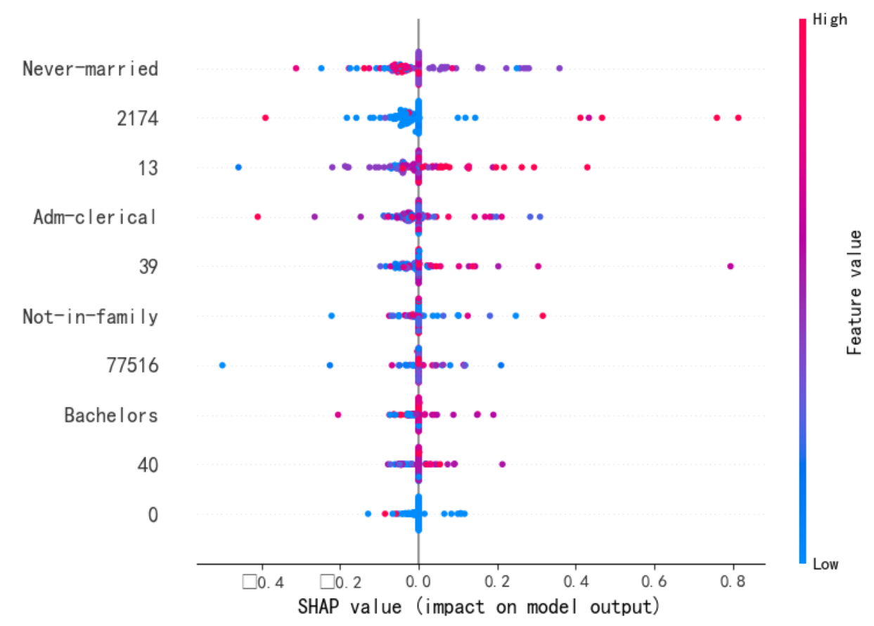
Step3：特征可解释性-SHAP

# pip show shap
import shap
shap.initjs()
explainer = shap.KernelExplainer(clf.predict, X_train)

X_test_ = X_test[1:100,:]
shap_values = explainer.shap_values(X_test_, nsamples=20)
print(shap_values)

X_test_ = pd.DataFrame(X_test_,columns=features)
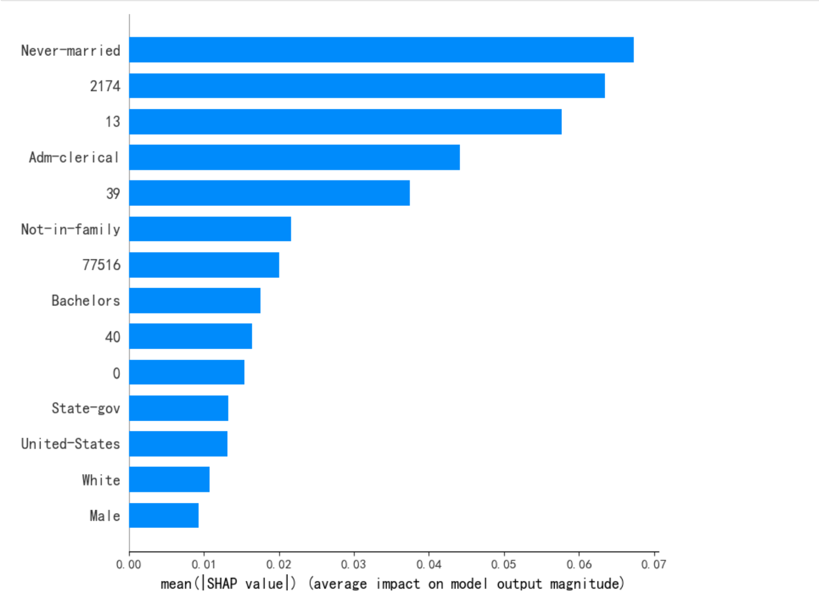
shap.summary_plot(shap_values, X_test_, plot_type = 'violin', max_display=10) # dot violin

shap.summary_plot(shap_values, X_test_, plot_type="bar") #[class_index]

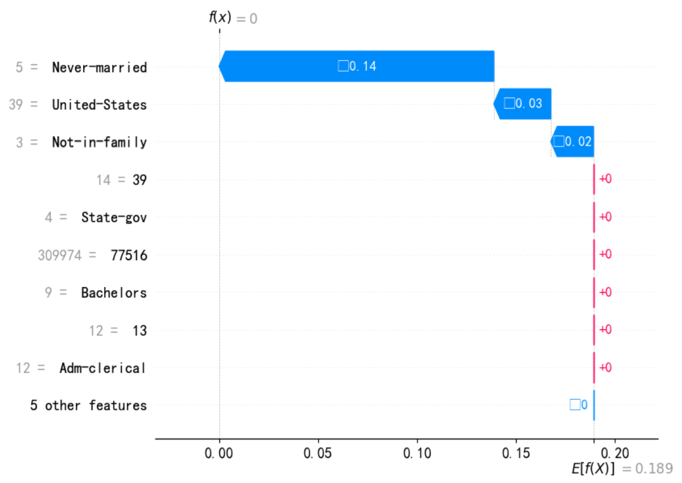
print(f"--- 解释样本 {idx} 的瀑布图 ---")

shap.waterfall_plot(
    shap.Explanation(
        values=shap_values[idx,:], # shap_values[class_index][idx,:],
        base_values=explainer.expected_value, # explainer.expected_value[class_index]
        data=X_test_.iloc[idx,:],
        feature_names=X_test_.columns.tolist()
    )
)

三、参考

github: https://github.com/dreamquark-ai/tabnet

https://mp.weixin.qq.com/s/6tdSoOOc7I7v-LSyGZ96rA

https://7568.github.io/2021/11/26/tabnet.html

https://zhuanlan.zhihu.com/p/152211918

shap:https://colab.research.google.com/drive/1bAXxurZEWfkCTyPeJn0YbHMrSKbneOKL?usp=sharing#scrollTo=C9qTb-lhNzVH

调优：https://www.kaggle.com/code/neilgibbons/tuning-tabnet-with-optuna/notebook（ReduceLROnPlateau）；https://www.kaggle.com/code/optimo/the-beauty-of-tabnet-a-simple-baseline（OneCycleLR）