一、理论部分

相关论文：Generative Adversarial Nets
摘要：We propose a new framework for estimating generative models via an adversar-ial process, in which we simultaneously train two models: a generative model G that captures the data distribution, and a discriminative model D that estimates the probability that a sample came from the training data rather than G. The train-ing procedure for G is to maximize the probability of D making a mistake. This framework corresponds to a minimax two-player game. In the space of arbitrary functions G and D, a unique solution exists, with G recovering the training data distribution and D equal to everywhere. In the case where G and D are defined by multilayer perceptrons, the entire system can be trained with backpropagation. There is no need for any Markov chains or unrolled approximate inference net-works during either training or generation of samples. Experiments demonstrate the potential of the framework through qualitative and quantitative evaluation of thegenerated samples.

---

1.1 基本原理

生成对抗网络（Generative Adversarial Network, GAN）是由 Ian Goodfellow 等人在 2014 年 提出的一种深度学习模型，主要用于生成逼真的数据（如图像、音频、文本等）。

GAN 的核心思想是通过两个神经网络相互对抗（生成器 vs. 判别器）来提升生成数据的质量。

• 生成器（Generator）：将随机噪声转换为逼真数据（如图像）
• 判别器（Discriminator）：区分真实数据与生成数据

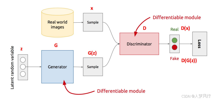
二者通过对抗训练共同提升，最终生成器能生成以假乱真的数据

---

1.2 损失函数

• 判别器损失：
  $L_D=-{\mathbb{E}}_{x\sim p_{data}}[\log D(x)]-{\mathbb{E}}_{z\sim p_z}[\log (1-D(G(z)))]$
• 生成器损失：
  $L_G=-{\mathbb{E}}_{z\sim p_z}[\log D(G(z))]\text{(或使用 }{L}_G={\mathbb{E}}_{z\sim p_z}[\log (1-D(G(z)))]$

---

1.3 训练流程

---

1.4 GAN的常见问题与解决方案

问题	原因	解决方案
模式崩溃（Mode Collapse）	生成器只生成少数样本	使用Mini-batch Discriminator
训练不稳定	梯度消失/爆炸	WGAN-GP，TTUR
生成质量差	网络容量不足	使用更深网络（如DCGAN）

---

1.5 进阶方向

1. Conditional GAN：加入标签信息控制生成内容
2. CycleGAN：无配对图像风格转换
3. StyleGAN：高分辨率人脸生成

通过调整网络结构和训练策略，GAN可应用于图像生成、超分辨率、数据增强等多个领域

---

二、代码实现

2.1 导包

import torch
import torch.nn as nn
from torch.utils.data import DataLoader
from torchvision import datasets, transforms
from torchvision.utils import save_image

import os
import numpy as np
import matplotlib.pyplot as plt
from tqdm.notebook import tqdm  
from torchsummary import summary

# 判断是否存在可用的GPU
device=torch.device("cuda:0" if torch.cuda.is_available() else "cpu")

2.2 数据加载和处理

# 加载 MNIST 数据集
def load_data(batch_size=64,img_shape=(1,28,28)):
    transform = transforms.Compose([
        transforms.Resize((img_shape[1],img_shape[2])),
        transforms.ToTensor(),  # 将图像转换为张量
        transforms.Normalize((0.5,), (0.5,))  # 归一化
    ])
    
    # 下载训练集和测试集
    train_dataset = datasets.MNIST(root='./data', train=True, download=True, transform=transform)
    test_dataset = datasets.MNIST(root='./data', train=False, download=True, transform=transform)
    
    # 创建 DataLoader
    train_loader = DataLoader(dataset=train_dataset, batch_size=batch_size, shuffle=True)
    test_loader = DataLoader(dataset=test_dataset, batch_size=batch_size, shuffle=False)
    return train_loader, test_loader

2.3 构建生成器

latent_dim 是生成对抗网络（GAN）中一个关键的超参数，表示 潜在空间（Latent Space）的维度，即生成器输入噪声向量的长度。

---

1. 核心概念

• 定义：latent_dim 决定了生成器输入噪声向量 z 的维度（通常为100-512维）
• 数学表示： z ∈ $R^{latent\_\dim }$，例如 latent_dim=100 时，z 是一个100维的随机向量
• 作用： 控制生成器输入的自由度，影响生成样本的多样性和质量

---

2. 典型取值

应用场景	推荐值	说明
小型图像（28x28）	50-100	MNIST/Fashion-MNIST等
中型图像（128x128）	100-256	CIFAR-10/小型人脸数据集
高清图像（256x256+）	256-512	CelebA/HQ等

---

3. 调整建议

• 增大 latent_dim：

  • 👍 提高生成多样性
  • 👎 可能增加训练难度（需更多数据/更长训练时间）

• 减小 latent_dim：

  • 👍 加速训练，降低模式崩溃风险
  • 👎 可能限制生成能力

---

4. 与其他参数的关系

参数	交互影响
batch_size	大batch需配合足够大的latent_dim
generator_capacity	高容量生成器可支持更大维度
dataset_complexity	复杂数据集需要更高维度

---

5. 可视化理解

---

7. 研究支持

• DCGAN论文 推荐 latent_dim=100 作为基准值
• StyleGAN 使用 latent_dim=512 以实现精细控制

---

通过合理调整 latent_dim，你可以平衡生成质量与训练效率。通常建议从 100 开始，根据生成效果逐步调整

class Generator(nn.Module):
    """生成器"""
    def __init__(self, latent_dim=100, img_shape=(1,28,28)):
        super(Generator,self).__init__()
        self.img_shape = img_shape  # 存储目标图片形状
        
        # 网络块
        def block(in_feat,out_feat,normalize=True):
            layers=[nn.Linear(in_feat,out_feat)]
            if normalize:
                #实践发现：对于生成器，较高的动量（如0.5-0.8）有时能提升生成多样性
                layers.append(nn.BatchNorm1d(out_feat,momentum = 0.8)) 
            layers.append(nn.LeakyReLU(negative_slope=0.2,inplace=True))
            return layers
            
        self.model = nn.Sequential(                       
            *block(latent_dim, 128,normalize=False),   # 输入：latent_dim维噪声
            *block(128, 256),
            *block(256, 512),
            *block(512,1024),
            nn.Linear(1024, int(np.prod(img_shape))), # 输出形状[B,C*H*W]
            nn.Tanh()  # 输出归一化到[-1,1]
        )

    def forward(self, z):
        img=self.model(z) # [B,C*H*W],2维数据
        img=img.view(img.shape[0],*self.img_shape) # 2维->4维[B,C,H,W]
        return img

• 打印生成器模型结构（一）

model_G = Generator().to(device)
# 打印模型摘要
summary(model_G, input_size=(100,)) 

----------------------------------------------------------------
        Layer (type)               Output Shape         Param #
================================================================
            Linear-1                  [-1, 128]          12,928
         LeakyReLU-2                  [-1, 128]               0
            Linear-3                  [-1, 256]          33,024
       BatchNorm1d-4                  [-1, 256]             512
         LeakyReLU-5                  [-1, 256]               0
            Linear-6                  [-1, 512]         131,584
       BatchNorm1d-7                  [-1, 512]           1,024
         LeakyReLU-8                  [-1, 512]               0
            Linear-9                 [-1, 1024]         525,312
      BatchNorm1d-10                 [-1, 1024]           2,048
        LeakyReLU-11                 [-1, 1024]               0
           Linear-12                  [-1, 784]         803,600
             Tanh-13                  [-1, 784]               0
================================================================
Total params: 1,510,032
Trainable params: 1,510,032
Non-trainable params: 0
----------------------------------------------------------------
Input size (MB): 0.00
Forward/backward pass size (MB): 0.05
Params size (MB): 5.76
Estimated Total Size (MB): 5.82
----------------------------------------------------------------

• 打印生成器模型结构（二）

z = torch.randn(64,100).to(device)
for layer in model_G.model:
    z=layer(z)
    print(f"{layer.__class__.__name__} --> Output shape={tuple(z.shape)}")

Linear --> Output shape=(64, 128)
LeakyReLU --> Output shape=(64, 128)
Linear --> Output shape=(64, 256)
BatchNorm1d --> Output shape=(64, 256)
LeakyReLU --> Output shape=(64, 256)
Linear --> Output shape=(64, 512)
BatchNorm1d --> Output shape=(64, 512)
LeakyReLU --> Output shape=(64, 512)
Linear --> Output shape=(64, 1024)
BatchNorm1d --> Output shape=(64, 1024)
LeakyReLU --> Output shape=(64, 1024)
Linear --> Output shape=(64, 784)
Tanh --> Output shape=(64, 784)

2.4 构建判别器

class Discriminator(nn.Module):
    """判别器"""
    def __init__(self,img_shape=(1,28,28)):
        super(Discriminator, self).__init__()

        self.model = nn.Sequential(
            nn.Linear(int(np.prod(img_shape)), 512),
            nn.LeakyReLU(0.2, inplace=True),
            nn.Linear(512, 256),
            nn.LeakyReLU(0.2, inplace=True),
            nn.Linear(256, 1),
            # nn.Sigmoid(), 无需归一到[0,1](概率值),
            # 使用nn.BCEWithLogitsLoss()，它结合了 Sigmoid + BCELoss，且数值更稳定
        )

    def forward(self, img):
        # 将输入图片展平
        img_flat = img.view(img.size(0), -1) # 4维[B,C,H,W]->2维[B,C*H*W]
        
        # 样本的真实性
        validity = self.model(img_flat) 
        return validity # [B,1]

• 打印判别器模型结构（一）

model_D = Discriminator().to(device)
# 打印模型摘要
summary(model_D, input_size=(1,28,28)) 

----------------------------------------------------------------
        Layer (type)               Output Shape         Param #
================================================================
            Linear-1                  [-1, 512]         401,920
         LeakyReLU-2                  [-1, 512]               0
            Linear-3                  [-1, 256]         131,328
         LeakyReLU-4                  [-1, 256]               0
            Linear-5                    [-1, 1]             257
================================================================
Total params: 533,505
Trainable params: 533,505
Non-trainable params: 0
----------------------------------------------------------------
Input size (MB): 0.00
Forward/backward pass size (MB): 0.01
Params size (MB): 2.04
Estimated Total Size (MB): 2.05
----------------------------------------------------------------

• 打印判别器模型结构（二）

img = torch.randn(64,1,28,28).to(device)
# 将输入图片展平
img = img.view(img.size(0), -1) # 4维[B,C,H,W]->2维[B,C*H*W]
for layer in model_D.model:
    img=layer(img)
    print(f"{layer.__class__.__name__} --> Output shape={tuple(img.shape)}")

Linear --> Output shape=(64, 512)
LeakyReLU --> Output shape=(64, 512)
Linear --> Output shape=(64, 256)
LeakyReLU --> Output shape=(64, 256)
Linear --> Output shape=(64, 1)

2.5 训练和保存模型

# 设置超参数
batch_size = 64
epochs = 200
lr= 2e-4
latent_dim=100 # 生成器输入噪声向量的长度(维数)
sample_interval=400 #每400次迭代保存生成样本

os.makedirs("./img/gan_mlp_mnist", exist_ok=True) # 存放生成样本目录
os.makedirs("./model", exist_ok=True) #模型存放目录

# 设置图片形状1*28*28
img_c,img_h,img_w=1,28,28
img_shape = (img_c,img_h,img_w)

# 加载数据
train_loader,_= load_data(batch_size=batch_size,img_shape=img_shape)

# 实例化生成器G、判别器D
G=Generator().to(device)
D=Discriminator().to(device)


# 设置优化器
optimizer_G = torch.optim.Adam(G.parameters(), lr=lr, betas=(0.5, 0.999))
optimizer_D = torch.optim.Adam(D.parameters(), lr=lr, betas=(0.5, 0.999))

# 损失函数
loss_fn=nn.BCEWithLogitsLoss()

# 开始训练
loader_len=len(train_loader) #训练加载器的长度
for epoch in range(epochs):
     #记录生成器G和判别器D的总损失(1个 epoch 内)
    gen_loss_sum,dis_loss_sum=0.0,0.0
    
    loop = tqdm(train_loader, desc=f"第{epoch+1}轮")
    for i, (real_imgs, _) in enumerate(loop):
        real_imgs=real_imgs.to(device)  # [B,C,H,W]
        # -----------------
        #  训练生成器
        # -----------------

        # 获取噪声样本[B,latent_dim]
        z=torch.normal(0,1,size=(real_imgs.shape[0],latent_dim),device=device)  #从正态分布中抽样

        # 更新生成器参数
        optimizer_G.zero_grad() #梯度清零
        gen_imgs=G(z) #生成一个批量的图片
        gen_loss=loss_fn(D(gen_imgs),torch.ones_like(D(gen_imgs))) #计算生成器损失
        gen_loss.backward() #反向传播,计算梯度
        optimizer_G.step()  #更新生成器  

        # -----------------
        #  训练判断器
        # -----------------
        optimizer_D.zero_grad() #梯度清零
        
        # 计算判断器损失=(判断真实图片损失+判断生成图片损失)/2
        real_loss=loss_fn(D(real_imgs),torch.ones_like(D(real_imgs)))
        fake_loss=loss_fn(D(gen_imgs.detach()),torch.zeros_like(D(gen_imgs.detach())))
        dis_loss=(real_loss+fake_loss)/2.0

        # 更新判断器参数
        dis_loss.backward() #反向传播,计算梯度
        optimizer_D.step()  #更新判断器  

        
        # 对生成器和判别器每次迭代的损失进行累加
        gen_loss_sum+=gen_loss
        dis_loss_sum+=dis_loss

        # 每 sample_interval 次迭代保存生成样本
        batches_done = epoch * loader_len + i
        if batches_done % sample_interval == 0:
            save_image(gen_imgs.data[:25], f"./img/gan_mlp_mnist/{epoch}_{i}.png", nrow=5, normalize=True)
            # 更新进度条
            loop.set_postfix(mean_gen_loss=f"{gen_loss_sum/(loop.n + 1):.8f}",mean_dis_loss=f"{dis_loss_sum/(loop.n + 1):.8f}")


#仅保存模型的参数（权重和偏置）,灵活性高，可以在不同的模型结构之间加载参数
torch.save(G.state_dict(), "./model/G_MLP.pth") 
torch.save(D.state_dict(), "./model/D_MLP.pth") 

2.6 训练生成过程

from PIL import Image

def create_gif(img_dir="./img/gan_mlp_mnist", output_file="./img/gan_mlp_mnist/gen_figure.gif", duration=100):
    images = []
    img_paths = [f for f in os.listdir(img_dir) if f.endswith(".png")]
    
    # 自定义排序：按 "x_y.png" 的 x 和 y 排序
    img_paths_sorted = sorted(
        img_paths,
        key=lambda x: (
            int(x.split('_')[0]),  # 第一个数字（如 0_400.png 的 0）
            int(x.split('_')[1].split('.')[0])  # 第二个数字（如 0_400.png 的 400）
        )
    )
    
    for img_file in img_paths_sorted:
        img = Image.open(os.path.join(img_dir, img_file))
        images.append(img)
    
    images[0].save(output_file, save_all=True, append_images=images[1:], 
                  duration=duration, loop=0)
    print(f"GIF已保存至 {output_file}")
create_gif()

2.7 模型加载和生成

#载入训练好的模型
G = Generator() # 定义模型结构
G.load_state_dict(torch.load("./model/G_MLP.pth",weights_only=True,map_location=device)) # 加载保存的参数
G.to(device) # 将模型移动到设备（GPU 或 CPU）
G.eval() # 将模型设置为评估模式

#抽取噪声数据
z=torch.normal(0,1,size=(10,100),device=device)
#生成假样本
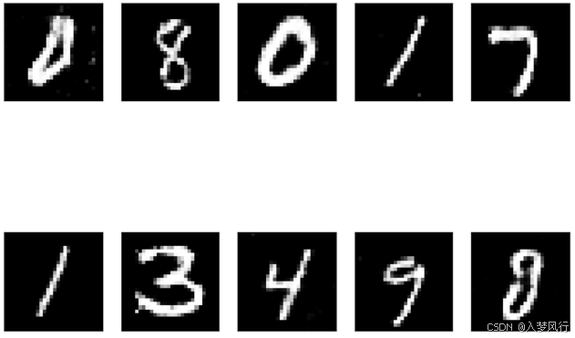
gen_img=G(z).view(-1,28,28) # 4维->3维
gen_img=gen_img.detach().cpu().numpy()

#绘制
for i in range(10):
    plt.subplot(2,5,i+1)
    plt.xticks([], [])
    plt.yticks([], [])
    plt.imshow(gen_img[i])
    plt.gray()
plt.show()