深度学习基础 - 多层感知机(MLP)通俗详解
想象一下你是一个水果摊老板输入信息(特征)顾客在看苹果的时间(0-10分钟)顾客摸苹果的次数(0-5次)今天的天气温度(0-40度)输出结果:是否购买(是/否)传统方法:你可能凭经验说:"如果看的时间>3分钟且摸的次数>2次,就会买"神经网络方法:让电脑自己从数据中学习这个规律!概念生活比喻在代码中的体现神经元小决策者权重特征重要性模型自动学习的参数偏置决策难易度每个神经元的bias参数激活函数开
什么是多层感知机?用生活案例来理解
基本概念比喻
想象一下你是一个水果摊老板,需要判断顾客是否会购买你的苹果:
输入信息(特征):
-
顾客在看苹果的时间(0-10分钟)
-
顾客摸苹果的次数(0-5次)
-
今天的天气温度(0-40度)
输出结果:是否购买(是/否)
传统方法:你可能凭经验说:"如果看的时间>3分钟且摸的次数>2次,就会买"
神经网络方法:让电脑自己从数据中学习这个规律!
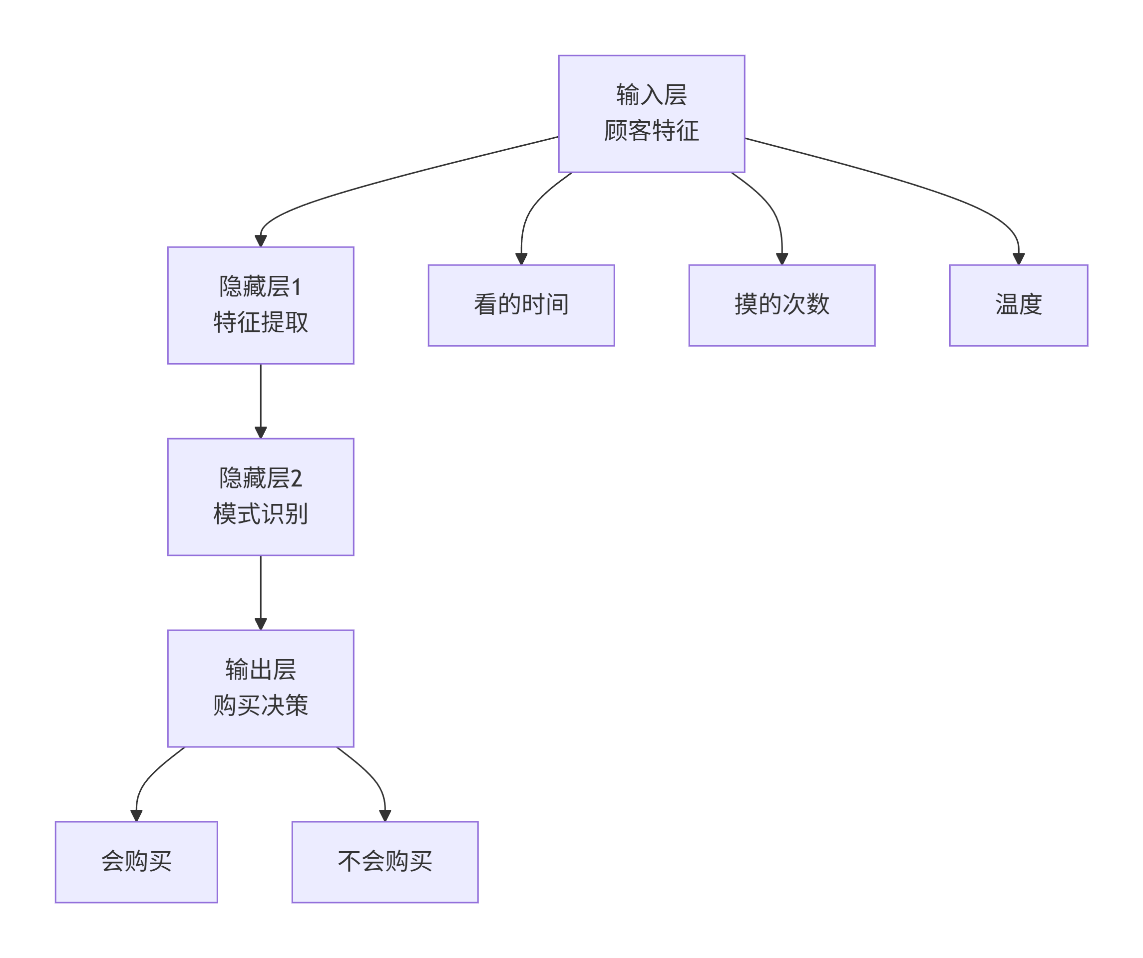
🎯 神经网络就像"智能决策工厂"
# 先看一个极简版的神经网络决策过程
def simple_neural_network(look_time, touch_count, temperature):
    # 第一层"思考":提取重要特征
    feature1 = look_time * 0.6 + touch_count * 0.3  # 关注度分数
    feature2 = temperature * 0.1 + touch_count * 0.4  # 购买意愿分数

    # 激活函数:决定是否"激活"这个特征
    activated_feature1 = max(0, feature1)  # ReLU激活函数
    activated_feature2 = max(0, feature2)

    # 输出层:综合判断
    buy_score = activated_feature1 * 0.7 + activated_feature2 * 0.5

    # 最终决策
    return "会购买" if buy_score > 0.5 else "不会购买"

# 测试
print(simple_neural_network(5, 3, 25))  # 看5分钟,摸3次,温度25度
神经网络核心概念详解
1. 神经元 - 像"小决策者"
每个神经元接收多个输入,进行加权计算,然后决定输出什么
import numpy as np

class SimpleNeuron:
    def __init__(self, weights, bias):
        self.weights = weights  # 权重:每个输入的重要程度
        self.bias = bias        # 偏置:决策的难易程度

    def forward(self, inputs):
        # 加权求和:inputs = [看的时间, 摸的次数, 温度]
        total = np.dot(inputs, self.weights) + self.bias

        # 激活函数:决定是否"激活"
        return max(0, total)  # ReLU函数

# 创建一个神经元:认为看的时间最重要,温度最不重要
neuron = SimpleNeuron(weights=[0.6, 0.3, 0.1], bias=-1.0)

# 测试神经元
customer_data = [5, 3, 25]  # 看5分钟,摸3次,温度25度
output = neuron.forward(customer_data)
print(f"神经元输出: {output}")
2. 激活函数 - 像"开关"
决定神经元是否被激活,引入非线性
import matplotlib.pyplot as plt

# 常见的激活函数
def relu(x):
    return max(0, x)

def sigmoid(x):
    return 1 / (1 + np.exp(-x))

def tanh(x):
    return np.tanh(x)

# 可视化激活函数
x = np.linspace(-5, 5, 100)
plt.figure(figsize=(12, 4))

plt.subplot(1, 3, 1)
plt.plot(x, [relu(i) for i in x])
plt.title('ReLU激活函数')
plt.grid(True)

plt.subplot(1, 3, 2)
plt.plot(x, [sigmoid(i) for i in x])
plt.title('Sigmoid激活函数')
plt.grid(True)

plt.subplot(1, 3, 3)
plt.plot(x, [tanh(i) for i in x])
plt.title('Tanh激活函数')
plt.grid(True)

plt.tight_layout()
plt.show()
3. 多层感知机结构 - 像"工厂流水线"
完整的可运行实例:水果购买预测
import numpy as np
import matplotlib.pyplot as plt
from sklearn.model_selection import train_test_split
from sklearn.preprocessing import StandardScaler
import tensorflow as tf
from tensorflow.keras import layers, models

# 设置随机种子保证结果可重现
np.random.seed(42)
tf.random.set_seed(42)

# 1. 生成模拟数据 - 200个顾客的购买记录
def generate_customer_data(num_samples=200):
    np.random.seed(42)

    # 生成特征
    look_time = np.random.uniform(0, 10, num_samples)  # 看的时间
    touch_count = np.random.randint(0, 6, num_samples)  # 摸的次数
    temperature = np.random.uniform(0, 40, num_samples)  # 温度

    # 生成标签(真实购买决策)- 基于一些简单规则
    # 规则:看的时间长、摸的次数多、温度适宜时更容易购买
    buy_probability = (look_time * 0.1 + touch_count * 0.3 +
                      np.where(temperature > 15, 0.2, 0) +
                      np.where(temperature < 30, 0.2, 0))

    # 添加一些噪声,让问题更有挑战性
    noise = np.random.normal(0, 0.2, num_samples)
    buy_probability += noise

    # 转换为二分类标签
    labels = (buy_probability > 0.5).astype(int)

    # 组合特征
    features = np.column_stack([look_time, touch_count, temperature])

    return features, labels

# 生成数据
print("生成顾客购买数据...")
X, y = generate_customer_data(200)

# 查看数据分布
print(f"数据形状: 特征{X.shape}, 标签{y.shape}")
print(f"购买人数: {np.sum(y)}, 未购买人数: {len(y) - np.sum(y)}")

# 数据可视化
plt.figure(figsize=(15, 5))

plt.subplot(1, 3, 1)
plt.scatter(X[y==0, 0], X[y==0, 1], alpha=0.7, label='未购买')
plt.scatter(X[y==1, 0], X[y==1, 1], alpha=0.7, label='购买')
plt.xlabel('看的时间(分钟)')
plt.ylabel('摸的次数')
plt.legend()
plt.title('看的时间 vs 摸的次数')

plt.subplot(1, 3, 2)
plt.scatter(X[y==0, 0], X[y==0, 2], alpha=0.7, label='未购买')
plt.scatter(X[y==1, 0], X[y==1, 2], alpha=0.7, label='购买')
plt.xlabel('看的时间(分钟)')
plt.ylabel('温度(度)')
plt.legend()
plt.title('看的时间 vs 温度')

plt.subplot(1, 3, 3)
plt.scatter(X[y==0, 1], X[y==0, 2], alpha=0.7, label='未购买')
plt.scatter(X[y==1, 1], X[y==1, 2], alpha=0.7, label='购买')
plt.xlabel('摸的次数')
plt.ylabel('温度(度)')
plt.legend()
plt.title('摸的次数 vs 温度')

plt.tight_layout()
plt.show()

# 2. 数据预处理
print("\n数据预处理...")
# 划分训练集和测试集
X_train, X_test, y_train, y_test = train_test_split(X, y, test_size=0.2, random_state=42)

# 数据标准化(重要!)
scaler = StandardScaler()
X_train_scaled = scaler.fit_transform(X_train)
X_test_scaled = scaler.transform(X_test)

print(f"训练集大小: {X_train_scaled.shape}")
print(f"测试集大小: {X_test_scaled.shape}")

# 3. 构建多层感知机模型
print("\n构建神经网络模型...")
def create_mlp_model():
    model = models.Sequential([
        # 输入层:3个特征(看的时间、摸的次数、温度)
        layers.Dense(16, activation='relu', input_shape=(3,), name='hidden_layer1'),
        layers.Dropout(0.2),  # 防止过拟合

        # 隐藏层:学习更复杂的模式
        layers.Dense(8, activation='relu', name='hidden_layer2'),
        layers.Dropout(0.2),

        # 输出层:二分类问题,使用sigmoid激活函数
        layers.Dense(1, activation='sigmoid', name='output_layer')
    ])
    return model

# 创建模型
model = create_mlp_model()

# 打印模型结构
print("模型结构:")
model.summary()

# 4. 编译模型
print("\n编译模型...")
model.compile(
    optimizer='adam',           # 优化器:自适应学习率
    loss='binary_crossentropy', # 损失函数:二分类问题
    metrics=['accuracy']        # 评估指标:准确率
)

# 5. 训练模型
print("\n开始训练模型...")
history = model.fit(
    X_train_scaled, y_train,
    epochs=100,                # 训练轮数
    batch_size=8,              # 批量大小
    validation_split=0.2,      # 验证集比例
    verbose=1                  # 显示训练进度
)

# 6. 评估模型
print("\n评估模型性能...")
train_loss, train_accuracy = model.evaluate(X_train_scaled, y_train, verbose=0)
test_loss, test_accuracy = model.evaluate(X_test_scaled, y_test, verbose=0)

print(f"训练集准确率: {train_accuracy:.4f}")
print(f"测试集准确率: {test_accuracy:.4f}")

# 7. 可视化训练过程
plt.figure(figsize=(12, 4))

plt.subplot(1, 2, 1)
plt.plot(history.history['accuracy'], label='训练准确率')
plt.plot(history.history['val_accuracy'], label='验证准确率')
plt.xlabel('训练轮数')
plt.ylabel('准确率')
plt.legend()
plt.title('训练和验证准确率')

plt.subplot(1, 2, 2)
plt.plot(history.history['loss'], label='训练损失')
plt.plot(history.history['val_loss'], label='验证损失')
plt.xlabel('训练轮数')
plt.ylabel('损失')
plt.legend()
plt.title('训练和验证损失')

plt.tight_layout()
plt.show()

# 8. 使用模型进行预测
print("\n使用模型进行预测...")

# 新顾客数据
new_customers = np.array([
    [8, 4, 25],   # 看8分钟,摸4次,温度25度 → 很可能购买
    [1, 0, 10],   # 看1分钟,没摸,温度10度 → 很可能不购买
    [5, 2, 20],   # 看5分钟,摸2次,温度20度 → 可能购买
])

# 标准化新数据
new_customers_scaled = scaler.transform(new_customers)

# 预测
predictions = model.predict(new_customers_scaled)
buy_probabilities = predictions.flatten()

print("\n预测结果:")
for i, (customer, prob) in enumerate(zip(new_customers, buy_probabilities)):
    decision = "会购买" if prob > 0.5 else "不会购买"
    confidence = prob if prob > 0.5 else 1 - prob
    print(f"顾客{i+1}: 看{customer[0]:.1f}分钟, 摸{customer[1]}次, 温度{customer[2]}度")
    print(f"  预测: {decision} (置信度: {confidence:.2%})")
    print()

# 9. 理解模型学到的规律
print("分析模型学到的规律...")

# 获取第一层权重
first_layer_weights = model.layers[0].get_weights()[0]
feature_names = ['看的时间', '摸的次数', '温度']

print("\n第一层神经元权重(特征重要性):")
for i in range(first_layer_weights.shape[1]):
    print(f"神经元{i+1}: ", end="")
    for j in range(3):
        importance = first_layer_weights[j, i]
        print(f"{feature_names[j]}: {importance:+.3f}  ", end="")
    print()

# 10. 模型决策边界可视化(简化版)
def plot_decision_boundary_simplified():
    """简化版的决策边界可视化"""
    # 固定一个特征,可视化另外两个特征的决策边界
    fixed_temperature = 20  # 固定温度为20度

    # 生成网格数据
    look_range = np.linspace(0, 10, 50)
    touch_range = np.linspace(0, 5, 50)
    Look, Touch = np.meshgrid(look_range, touch_range)

    # 创建测试数据
    test_data = np.column_stack([
        Look.ravel(),
        Touch.ravel(),
        np.full(Look.ravel().shape, fixed_temperature)
    ])

    # 标准化并预测
    test_data_scaled = scaler.transform(test_data)
    predictions = model.predict(test_data_scaled)
    Z = predictions.reshape(Look.shape)

    # 绘图
    plt.figure(figsize=(10, 8))
    contour = plt.contourf(Look, Touch, Z, levels=20, alpha=0.6, cmap='RdYlBu')
    plt.colorbar(contour, label='购买概率')

    # 绘制原始数据点
    scatter = plt.scatter(X[:, 0], X[:, 1], c=y, cmap='RdYlBu', edgecolors='black', alpha=0.7)
    plt.colorbar(scatter, label='真实标签')

    plt.xlabel('看的时间(分钟)')
    plt.ylabel('摸的次数')
    plt.title(f'决策边界可视化 (温度固定为{fixed_temperature}度)')
    plt.grid(True, alpha=0.3)
    plt.show()

# 绘制决策边界
plot_decision_boundary_simplified()

print("\n🎉 恭喜!你已经完成了第一个神经网络项目的完整流程!")
代码运行结果解读
当你运行上面的代码时,你会看到:
-
数据分布图:显示不同特征之间的关系
-
模型训练过程:看到准确率逐渐提高,损失逐渐降低
-
预测结果:模型对新顾客的购买行为预测
-
决策边界:可视化模型如何区分"购买"和"不购买"
核心概念总结
|
概念 |
生活比喻 |
在代码中的体现 |
|---|---|---|
| 神经元 |
小决策者 |
layers.Dense() |
| 权重 |
特征重要性 |
模型自动学习的参数 |
| 偏置 |
决策难易度 |
每个神经元的bias参数 |
| 激活函数 |
开关机制 |
activation='relu'
或 |
| 损失函数 |
犯错程度 |
binary_crossentropy |
| 优化器 |
学习方法 |
optimizer='adam' |
|
** epoch** |
学习遍数 |
整个数据集训练的次数 |
💡 学习建议
-
先运行代码:看到实际效果,建立直观感受
-
修改参数:尝试改变神经元数量、层数、学习率等
-
观察变化:注意这些改变如何影响模型性能
-
理解原理:结合生活案例理解每个概念的意义
这个实例展示了从数据生成到模型训练、评估、预测的完整流程,是理解深度学习基础的最佳起点!
更多信息请关注微信公众号:AI弟

魔乐社区(Modelers.cn) 是一个中立、公益的人工智能社区,提供人工智能工具、模型、数据的托管、展示与应用协同服务,为人工智能开发及爱好者搭建开放的学习交流平台。社区通过理事会方式运作,由全产业链共同建设、共同运营、共同享有,推动国产AI生态繁荣发展。
更多推荐


 5
5 0
0- 0


 已为社区贡献1条内容

所有评论(0)