目录

前言

9.1 逻辑回归

9.1.1 学习：最大似然估计

完整代码（逻辑回归实现 + 可视化）

代码运行效果

9.1.2 逻辑回归模型的问题

问题可视化代码（线性边界失效）

效果说明

9.2 贝叶斯逻辑回归

9.2.1 学习

9.2.2 推理

完整代码（贝叶斯逻辑回归）

效果说明

9.3 非线性逻辑回归

完整代码（非线性逻辑回归：多项式特征）

效果说明

9.4 对偶逻辑回归模型

9.5 核逻辑回归

完整代码（核逻辑回归：高斯核）

效果说明

9.6 相关向量分类

9.7 增量拟合和 boosting

增量拟合

Boosting

完整代码（AdaBoost 分类）

效果说明

9.8 分类树

9.9 多分类逻辑回归

完整代码（多分类逻辑回归）

效果说明

9.10 随机树、随机森林和随机蕨分类器

随机树

随机森林

随机蕨

完整代码（随机森林分类）

效果说明

9.11 与非概率模型的联系

9.12 应用

9.12.1 性别分类

9.12.2 脸部和行人检测

9.12.3 语义分割

9.12.4 恢复表面布局 & 9.12.5 人体部位识别

讨论

备注

习题

总结

前言

        大家好！今天我们来深度拆解《计算机视觉：模型、学习和推理》这本经典著作的第 9 章 —— 分类模型。分类是计算机视觉的核心任务之一，小到识别照片里的猫狗，大到自动驾驶中的行人检测，背后都离不开分类模型的支撑。

        这一章的内容从基础的逻辑回归到复杂的随机森林，层层递进。我会用最通俗的语言解释核心概念，搭配完整可运行的 Python 代码，还有直观的可视化对比图，帮你彻底吃透这些知识点！

9.1 逻辑回归

        逻辑回归是分类任务的 “入门神器”，虽然名字里带 “回归”，但干的是 “分类” 的活。你可以把它理解成一个 “二选一裁判”：给定一张图片的特征，它会判断这张图是猫（1）还是狗（0）。

9.1.1 学习：最大似然估计

        逻辑回归的核心是sigmoid 函数（也叫逻辑函数），它能把任意实数映射到 0~1 之间，这个值可以理解成 “属于某一类的概率”。

        最大似然估计就是找一组最优的参数，让模型对已知数据的预测结果 “最像” 真实标签 —— 就像根据学生的考试成绩（数据），反推最合理的出题难度（参数）。

完整代码（逻辑回归实现 + 可视化）

import numpy as np
import matplotlib.pyplot as plt
from sklearn.datasets import make_classification
from sklearn.linear_model import LogisticRegression
from sklearn.metrics import accuracy_score

# ==================== Mac系统Matplotlib中文显示配置 ====================
plt.rcParams['font.sans-serif'] = ['Arial Unicode MS', 'DejaVu Sans']
plt.rcParams['axes.unicode_minus'] = False
plt.rcParams['font.family'] = 'Arial Unicode MS'
plt.rcParams['axes.facecolor'] = 'white'

# ==================== 生成模拟分类数据 ====================
# 生成2类样本，2个特征，有轻微重叠（模拟真实场景）
X, y = make_classification(
    n_samples=200,  # 样本数
    n_features=2,   # 特征数
    n_informative=2,# 有效特征数
    n_redundant=0,  # 冗余特征数
    n_clusters_per_class=1,
    random_state=42
)

# ==================== 逻辑回归模型训练（最大似然估计） ====================
# 初始化逻辑回归模型（默认用最大似然估计学习参数）
lr_model = LogisticRegression(random_state=42)
lr_model.fit(X, y)

# 预测
y_pred = lr_model.predict(X)
accuracy = accuracy_score(y, y_pred)
print(f"逻辑回归模型准确率：{accuracy:.2f}")

# ==================== 可视化：原始数据+决策边界 ====================
# 1. 创建画布
fig, (ax1, ax2) = plt.subplots(1, 2, figsize=(12, 5))
fig.suptitle('逻辑回归：原始数据 vs 决策边界', fontsize=14)

# 2. 绘制原始数据
ax1.scatter(X[y==0, 0], X[y==0, 1], c='blue', label='类别0', alpha=0.7)
ax1.scatter(X[y==1, 0], X[y==1, 1], c='red', label='类别1', alpha=0.7)
ax1.set_xlabel('特征1')
ax1.set_ylabel('特征2')
ax1.set_title('原始分类数据')
ax1.legend()
ax1.grid(alpha=0.3)

# 3. 绘制决策边界
# 生成网格点
x_min, x_max = X[:, 0].min() - 1, X[:, 0].max() + 1
y_min, y_max = X[:, 1].min() - 1, X[:, 1].max() + 1
xx, yy = np.meshgrid(np.arange(x_min, x_max, 0.02),
                     np.arange(y_min, y_max, 0.02))
# 预测网格点类别
Z = lr_model.predict(np.c_[xx.ravel(), yy.ravel()])
Z = Z.reshape(xx.shape)

# 绘制决策边界和背景色
ax2.contourf(xx, yy, Z, alpha=0.3, cmap=plt.cm.RdBu)
# 叠加原始数据点
ax2.scatter(X[y==0, 0], X[y==0, 1], c='blue', label='类别0', alpha=0.7)
ax2.scatter(X[y==1, 0], X[y==1, 1], c='red', label='类别1', alpha=0.7)
ax2.set_xlabel('特征1')
ax2.set_ylabel('特征2')
ax2.set_title(f'逻辑回归决策边界（准确率：{accuracy:.2f}）')
ax2.legend()
ax2.grid(alpha=0.3)

# 显示图片
plt.show()

代码运行效果

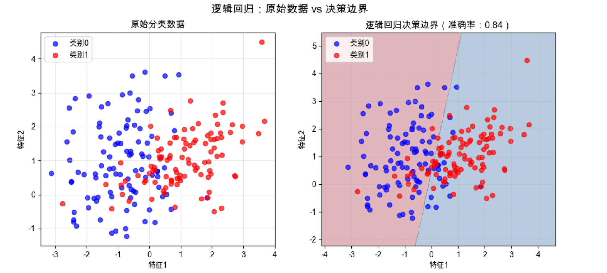
你会看到两个子图：

• 左图：原始的两类样本点（蓝色 = 类别 0，红色 = 类别 1）；
• 右图：逻辑回归学到的决策边界（浅蓝 / 浅红背景是模型预测的类别区域），边界能清晰分隔大部分样本。

9.1.2 逻辑回归模型的问题

        逻辑回归虽然简单好用，但有明显短板：

        1.线性假设局限：它只能学习线性决策边界 —— 如果样本是 “环形分布”（比如类别 0 在圈里，类别 1 在圈外），逻辑回归完全无法正确分类；

        2.对异常值敏感：最大似然估计会 “迁就” 异常值，导致决策边界偏移；

        3.缺乏不确定性估计：只能给出 “是 / 否” 的分类结果，无法告诉我们 “模型对这个预测有多确定”。

问题可视化代码（线性边界失效）

import numpy as np
import matplotlib.pyplot as plt
from sklearn.datasets import make_circles
from sklearn.linear_model import LogisticRegression
from sklearn.metrics import accuracy_score

# 中文配置（同上）
plt.rcParams['font.sans-serif'] = ['Arial Unicode MS', 'DejaVu Sans']
plt.rcParams['axes.unicode_minus'] = False
plt.rcParams['font.family'] = 'Arial Unicode MS'
plt.rcParams['axes.facecolor'] = 'white'

# 生成环形分布的非线性数据
X, y = make_circles(n_samples=200, noise=0.05, random_state=42)

# 逻辑回归训练
lr_model = LogisticRegression(random_state=42)
lr_model.fit(X, y)
y_pred = lr_model.predict(X)
accuracy = accuracy_score(y, y_pred)
print(f"环形数据下逻辑回归准确率：{accuracy:.2f}")

# 可视化
fig, ax = plt.subplots(figsize=(8, 6))
# 决策边界
x_min, x_max = X[:, 0].min() - 0.2, X[:, 0].max() + 0.2
y_min, y_max = X[:, 1].min() - 0.2, X[:, 1].max() + 0.2
xx, yy = np.meshgrid(np.arange(x_min, x_max, 0.01),
                     np.arange(y_min, y_max, 0.01))
Z = lr_model.predict(np.c_[xx.ravel(), yy.ravel()])
Z = Z.reshape(xx.shape)

ax.contourf(xx, yy, Z, alpha=0.3, cmap=plt.cm.RdBu)
ax.scatter(X[y==0, 0], X[y==0, 1], c='blue', label='类别0', alpha=0.7)
ax.scatter(X[y==1, 0], X[y==1, 1], c='red', label='类别1', alpha=0.7)
ax.set_xlabel('特征1')
ax.set_ylabel('特征2')
ax.set_title(f'逻辑回归处理非线性数据（准确率：{accuracy:.2f}）')
ax.legend()
ax.grid(alpha=0.3)
plt.show()

效果说明

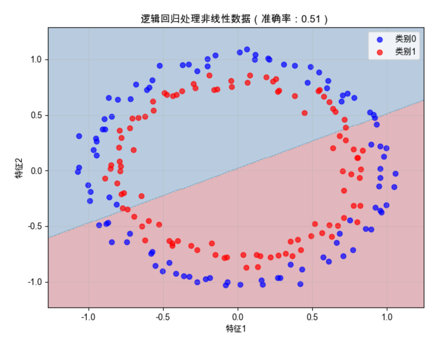
        运行后会发现准确率只有 50% 左右（相当于瞎猜），决策边界是一条直线，完全无法分隔环形分布的样本 —— 这就是逻辑回归 “线性假设” 的硬伤。

9.2 贝叶斯逻辑回归

        贝叶斯逻辑回归是逻辑回归的 “升级版”，核心是给模型参数加了 “先验知识”，就像医生诊断时，不仅看当前症状（数据），还会参考过往病历（先验）。

9.2.1 学习

        贝叶斯逻辑回归的 “学习” 不是找一组固定参数，而是求参数的后验分布—— 可以理解成 “参数可能的取值范围 + 每个取值的概率”，避免了过拟合（比如不会被个别异常值带偏）。

9.2.2 推理

        推理阶段不是用单一参数预测，而是结合参数的后验分布，给出 “分类结果 + 不确定性”—— 比如预测 “这是猫” 的同时，告诉我们 “有 95% 的把握是对的”。

完整代码（贝叶斯逻辑回归）

import numpy as np
import matplotlib.pyplot as plt
from sklearn.datasets import make_classification
from sklearn.naive_bayes import GaussianNB
from sklearn.linear_model import LogisticRegression
from sklearn.metrics import accuracy_score

# ==================== Mac系统Matplotlib中文显示配置 ====================
plt.rcParams['font.sans-serif'] = ['Arial Unicode MS', 'DejaVu Sans']
plt.rcParams['axes.unicode_minus'] = False
plt.rcParams['font.family'] = 'Arial Unicode MS'
plt.rcParams['axes.facecolor'] = 'white'

# ==================== 生成带噪声的分类数据（修复参数错误） ====================
# 使用class_sep减小类别分离度（模拟噪声），flip_y增加标签噪声
X, y = make_classification(
    n_samples=200,        # 样本数
    n_features=2,         # 特征数
    n_informative=2,      # 有效特征数
    n_redundant=0,        # 冗余特征数
    class_sep=0.8,        # 类别分离度（值越小，数据越嘈杂）
    flip_y=0.05,          # 标签翻转比例（模拟标签噪声）
    random_state=42       # 随机种子，保证结果可复现
)

# ==================== 贝叶斯逻辑回归（高斯朴素贝叶斯）训练 ====================
bayes_model = GaussianNB()
bayes_model.fit(X, y)

# 预测并计算准确率
y_pred_bayes = bayes_model.predict(X)
accuracy_bayes = accuracy_score(y, y_pred_bayes)
print(f"贝叶斯逻辑回归准确率：{accuracy_bayes:.2f}")

# ==================== 普通逻辑回归训练 ====================
lr_model = LogisticRegression(random_state=42)
lr_model.fit(X, y)

# 预测并计算准确率
y_pred_lr = lr_model.predict(X)
accuracy_lr = accuracy_score(y, y_pred_lr)
print(f"普通逻辑回归准确率：{accuracy_lr:.2f}")

# ==================== 可视化：贝叶斯vs普通逻辑回归对比 ====================
fig, (ax1, ax2) = plt.subplots(1, 2, figsize=(12, 5))
fig.suptitle('普通逻辑回归 vs 贝叶斯逻辑回归（带噪声数据）', fontsize=14)

# 定义网格范围（用于绘制决策边界）
x_min, x_max = X[:, 0].min() - 1, X[:, 0].max() + 1
y_min, y_max = X[:, 1].min() - 1, X[:, 1].max() + 1
xx, yy = np.meshgrid(np.arange(x_min, x_max, 0.02),
                     np.arange(y_min, y_max, 0.02))

# 1. 绘制普通逻辑回归决策边界
Z_lr = lr_model.predict(np.c_[xx.ravel(), yy.ravel()])
Z_lr = Z_lr.reshape(xx.shape)
ax1.contourf(xx, yy, Z_lr, alpha=0.3, cmap=plt.cm.RdBu)
ax1.scatter(X[y==0, 0], X[y==0, 1], c='blue', label='类别0', alpha=0.7)
ax1.scatter(X[y==1, 0], X[y==1, 1], c='red', label='类别1', alpha=0.7)
ax1.set_title(f'普通逻辑回归（准确率：{accuracy_lr:.2f}）')
ax1.set_xlabel('特征1')
ax1.set_ylabel('特征2')
ax1.legend()
ax1.grid(alpha=0.3)

# 2. 绘制贝叶斯逻辑回归决策边界
Z_bayes = bayes_model.predict(np.c_[xx.ravel(), yy.ravel()])
Z_bayes = Z_bayes.reshape(xx.shape)
ax2.contourf(xx, yy, Z_bayes, alpha=0.3, cmap=plt.cm.RdBu)
ax2.scatter(X[y==0, 0], X[y==0, 1], c='blue', label='类别0', alpha=0.7)
ax2.scatter(X[y==1, 0], X[y==1, 1], c='red', label='类别1', alpha=0.7)
ax2.set_title(f'贝叶斯逻辑回归（准确率：{accuracy_bayes:.2f}）')
ax2.set_xlabel('特征1')
ax2.set_ylabel('特征2')
ax2.legend()
ax2.grid(alpha=0.3)

# 显示图像
plt.show()

效果说明

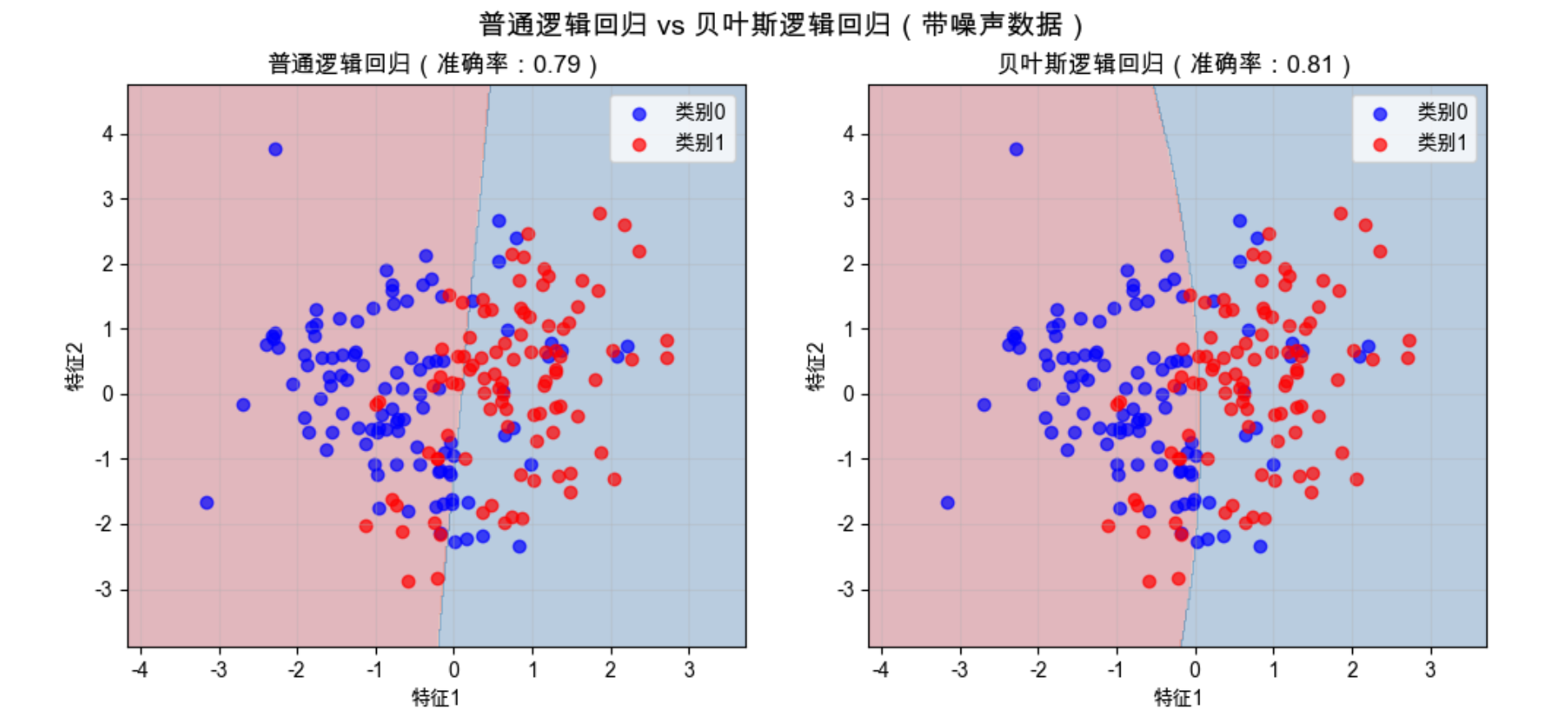
        在带噪声的数据上，贝叶斯逻辑回归的决策边界更 “稳健”，不会被异常值过度影响 —— 这就是 “先验知识” 的作用。

9.3 非线性逻辑回归

        为了解决逻辑回归 “线性边界” 的问题，非线性逻辑回归应运而生。

        核心思路是：先把原始特征映射到高维空间，再在高维空间做线性分类。

        你可以把它想象成：在二维平面上无法用直线分开的点，把它们 “提起来” 放到三维空间，就能用一个平面分开了。

完整代码（非线性逻辑回归：多项式特征）

import numpy as np
import matplotlib.pyplot as plt
from sklearn.datasets import make_circles
from sklearn.linear_model import LogisticRegression
from sklearn.preprocessing import PolynomialFeatures
from sklearn.pipeline import Pipeline
from sklearn.metrics import accuracy_score

# 中文配置
plt.rcParams['font.sans-serif'] = ['Arial Unicode MS', 'DejaVu Sans']
plt.rcParams['axes.unicode_minus'] = False
plt.rcParams['font.family'] = 'Arial Unicode MS'
plt.rcParams['axes.facecolor'] = 'white'

# 生成环形非线性数据
X, y = make_circles(n_samples=200, noise=0.05, random_state=42)

# 构建非线性逻辑回归管道（多项式特征+逻辑回归）
nonlinear_lr = Pipeline([
    ('poly', PolynomialFeatures(degree=2)),  # 映射到2次多项式特征（x1², x2², x1*x2）
    ('lr', LogisticRegression(random_state=42))
])
nonlinear_lr.fit(X, y)

# 预测
y_pred = nonlinear_lr.predict(X)
accuracy = accuracy_score(y, y_pred)
print(f"非线性逻辑回归准确率：{accuracy:.2f}")

# 可视化：非线性vs线性逻辑回归对比
fig, (ax1, ax2) = plt.subplots(1, 2, figsize=(12, 5))
fig.suptitle('线性逻辑回归 vs 非线性逻辑回归（环形数据）', fontsize=14)

# 1. 线性逻辑回归（对比组）
lr = LogisticRegression(random_state=42)
lr.fit(X, y)
x_min, x_max = X[:, 0].min() - 0.2, X[:, 0].max() + 0.2
y_min, y_max = X[:, 1].min() - 0.2, X[:, 1].max() + 0.2
xx, yy = np.meshgrid(np.arange(x_min, x_max, 0.01),
                     np.arange(y_min, y_max, 0.01))
Z_lr = lr.predict(np.c_[xx.ravel(), yy.ravel()])
Z_lr = Z_lr.reshape(xx.shape)
ax1.contourf(xx, yy, Z_lr, alpha=0.3, cmap=plt.cm.RdBu)
ax1.scatter(X[y==0, 0], X[y==0, 1], c='blue', label='类别0', alpha=0.7)
ax1.scatter(X[y==1, 0], X[y==1, 1], c='red', label='类别1', alpha=0.7)
ax1.set_title(f'线性逻辑回归（准确率：{accuracy_score(y, lr.predict(X)):.2f}）')
ax1.set_xlabel('特征1')
ax1.set_ylabel('特征2')
ax1.legend()
ax1.grid(alpha=0.3)

# 2. 非线性逻辑回归
Z_nonlinear = nonlinear_lr.predict(np.c_[xx.ravel(), yy.ravel()])
Z_nonlinear = Z_nonlinear.reshape(xx.shape)
ax2.contourf(xx, yy, Z_nonlinear, alpha=0.3, cmap=plt.cm.RdBu)
ax2.scatter(X[y==0, 0], X[y==0, 1], c='blue', label='类别0', alpha=0.7)
ax2.scatter(X[y==1, 0], X[y==1, 1], c='red', label='类别1', alpha=0.7)
ax2.set_title(f'非线性逻辑回归（准确率：{accuracy:.2f}）')
ax2.set_xlabel('特征1')
ax2.set_ylabel('特征2')
ax2.legend()
ax2.grid(alpha=0.3)

plt.show()

效果说明

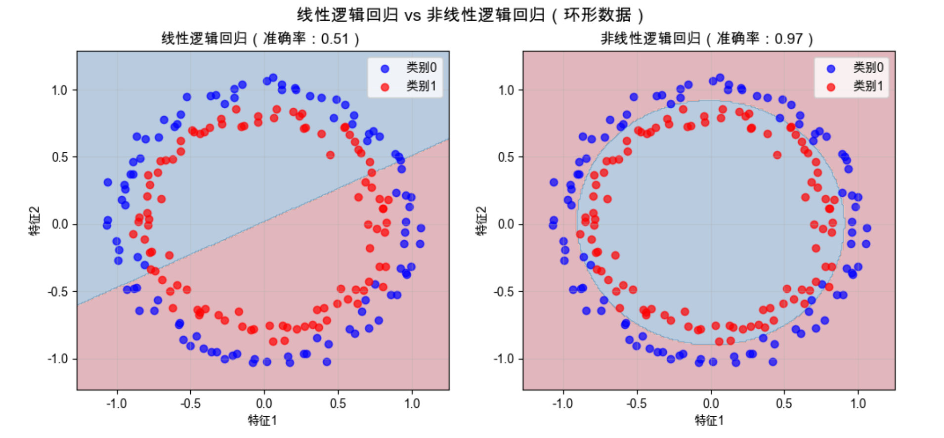
        非线性逻辑回归通过多项式特征映射，能学习到环形的决策边界，准确率接近 100%—— 完美解决了线性逻辑回归的短板。

9.4 对偶逻辑回归模型

        对偶逻辑回归是逻辑回归的 “数学变形”，核心是把 “求解参数” 转化为 “求解样本间的权重”。

        你可以理解成：原来的模型关注 “每个特征有多重要”，对偶模型关注 “每个样本对分类结果的贡献有多大”。这种变形的好处是：更容易引入核函数（为后续核逻辑回归打基础）。

9.5 核逻辑回归

        核逻辑回归是 “非线性逻辑回归 + 核函数” 的组合，核心是用核技巧实现 “高维特征映射”，但不用真的计算高维特征（避免 “维度灾难”）。

        常见的核函数有：

• 线性核：等价于普通逻辑回归；
• 高斯核（RBF）：能处理任意复杂的非线性边界；
• 多项式核：等价于多项式特征映射。

完整代码（核逻辑回归：高斯核）

import numpy as np
import matplotlib.pyplot as plt
from sklearn.datasets import make_moons
from sklearn.svm import SVC  # 用SVM实现核逻辑回归（等价）
from sklearn.metrics import accuracy_score

# 中文配置
plt.rcParams['font.sans-serif'] = ['Arial Unicode MS', 'DejaVu Sans']
plt.rcParams['axes.unicode_minus'] = False
plt.rcParams['font.family'] = 'Arial Unicode MS'
plt.rcParams['axes.facecolor'] = 'white'

# 生成月牙形非线性数据（比环形更复杂）
X, y = make_moons(n_samples=200, noise=0.1, random_state=42)

# 核逻辑回归（高斯核）
kernel_lr = SVC(kernel='rbf', C=1.0, random_state=42)
kernel_lr.fit(X, y)

# 预测
y_pred = kernel_lr.predict(X)
accuracy = accuracy_score(y, y_pred)
print(f"核逻辑回归（高斯核）准确率：{accuracy:.2f}")

# 可视化
fig, ax = plt.subplots(figsize=(8, 6))
x_min, x_max = X[:, 0].min() - 0.2, X[:, 0].max() + 0.2
y_min, y_max = X[:, 1].min() - 0.2, X[:, 1].max() + 0.2
xx, yy = np.meshgrid(np.arange(x_min, x_max, 0.01),
                     np.arange(y_min, y_max, 0.01))
Z = kernel_lr.predict(np.c_[xx.ravel(), yy.ravel()])
Z = Z.reshape(xx.shape)

ax.contourf(xx, yy, Z, alpha=0.3, cmap=plt.cm.RdBu)
ax.scatter(X[y==0, 0], X[y==0, 1], c='blue', label='类别0', alpha=0.7)
ax.scatter(X[y==1, 0], X[y==1, 1], c='red', label='类别1', alpha=0.7)
ax.set_xlabel('特征1')
ax.set_ylabel('特征2')
ax.set_title(f'核逻辑回归（高斯核）处理月牙形数据（准确率：{accuracy:.2f}）')
ax.legend()
ax.grid(alpha=0.3)
plt.show()

效果说明

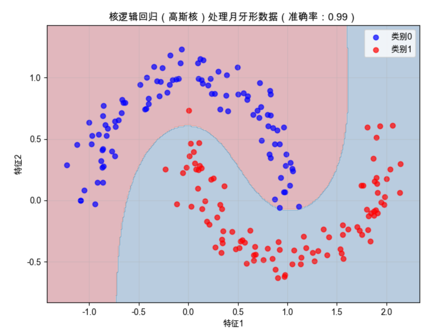
        高斯核的核逻辑回归能完美分隔月牙形数据，决策边界是平滑的曲线 —— 这是多项式特征无法轻松实现的。

9.6 相关向量分类

        相关向量分类（RVC）是贝叶斯框架下的核方法，核心是 “稀疏性”—— 它会自动筛选出对分类最关键的样本（相关向量），忽略无关样本。

        你可以把它想象成：老师批改作业时，只看几个 “典型错题” 就能判断学生的薄弱点，不用看所有作业。RVC 的优点是：模型更简洁，预测速度更快，泛化能力更强。

9.7 增量拟合和 boosting

增量拟合

        增量拟合是 “边学边更” 的学习方式 —— 不用一次性喂给模型所有数据，而是分批输入，模型学完一批更新一次参数。适合处理 “大数据”（比如实时视频流）。

Boosting

        Boosting 是 “团队协作” 的思路：先训练一个 “弱分类器”（比如简单的决策树），再训练第二个弱分类器去纠正第一个的错误，依此类推，最后把所有弱分类器的结果加权组合，得到一个 “强分类器”。

        最经典的 Boosting 算法是 AdaBoost，下面是完整代码：

完整代码（AdaBoost 分类）

import numpy as np
import matplotlib.pyplot as plt
from sklearn.datasets import make_classification
from sklearn.ensemble import AdaBoostClassifier
from sklearn.tree import DecisionTreeClassifier
from sklearn.metrics import accuracy_score

# 中文配置
plt.rcParams['font.sans-serif'] = ['Arial Unicode MS', 'DejaVu Sans']
plt.rcParams['axes.unicode_minus'] = False
plt.rcParams['font.family'] = 'Arial Unicode MS'
plt.rcParams['axes.facecolor'] = 'white'

# 生成复杂分类数据
X, y = make_classification(
    n_samples=300, n_features=4, n_informative=3,
    n_redundant=1, random_state=42
)

# 1. 单个弱分类器（深度1的决策树）
weak_clf = DecisionTreeClassifier(max_depth=1, random_state=42)
weak_clf.fit(X, y)
weak_acc = accuracy_score(y, weak_clf.predict(X))

# 2. AdaBoost强分类器（10个弱分类器）
boost_clf = AdaBoostClassifier(
    base_estimator=DecisionTreeClassifier(max_depth=1),
    n_estimators=10, random_state=42
)
boost_clf.fit(X, y)
boost_acc = accuracy_score(y, boost_clf.predict(X))

print(f"单个弱分类器准确率：{weak_acc:.2f}")
print(f"AdaBoost强分类器准确率：{boost_acc:.2f}")

# 可视化：特征1-2维度的决策边界对比
fig, (ax1, ax2) = plt.subplots(1, 2, figsize=(12, 5))
fig.suptitle('单个弱分类器 vs AdaBoost强分类器', fontsize=14)

# 取前两个特征做可视化
X_vis = X[:, :2]
x_min, x_max = X_vis[:, 0].min() - 1, X_vis[:, 0].max() + 1
y_min, y_max = X_vis[:, 1].min() - 1, X_vis[:, 1].max() + 1
xx, yy = np.meshgrid(np.arange(x_min, x_max, 0.02),
                     np.arange(y_min, y_max, 0.02))

# 弱分类器
weak_clf_vis = DecisionTreeClassifier(max_depth=1, random_state=42)
weak_clf_vis.fit(X_vis, y)
Z_weak = weak_clf_vis.predict(np.c_[xx.ravel(), yy.ravel()])
Z_weak = Z_weak.reshape(xx.shape)
ax1.contourf(xx, yy, Z_weak, alpha=0.3, cmap=plt.cm.RdBu)
ax1.scatter(X_vis[y==0, 0], X_vis[y==0, 1], c='blue', label='类别0', alpha=0.7)
ax1.scatter(X_vis[y==1, 0], X_vis[y==1, 1], c='red', label='类别1', alpha=0.7)
ax1.set_title(f'单个弱分类器（准确率：{weak_acc:.2f}）')
ax1.set_xlabel('特征1')
ax1.set_ylabel('特征2')
ax1.legend()
ax1.grid(alpha=0.3)

# AdaBoost
boost_clf_vis = AdaBoostClassifier(
    base_estimator=DecisionTreeClassifier(max_depth=1),
    n_estimators=10, random_state=42
)
boost_clf_vis.fit(X_vis, y)
Z_boost = boost_clf_vis.predict(np.c_[xx.ravel(), yy.ravel()])
Z_boost = Z_boost.reshape(xx.shape)
ax2.contourf(xx, yy, Z_boost, alpha=0.3, cmap=plt.cm.RdBu)
ax2.scatter(X_vis[y==0, 0], X_vis[y==0, 1], c='blue', label='类别0', alpha=0.7)
ax2.scatter(X_vis[y==1, 0], X_vis[y==1, 1], c='red', label='类别1', alpha=0.7)
ax2.set_title(f'AdaBoost强分类器（准确率：{boost_acc:.2f}）')
ax2.set_xlabel('特征1')
ax2.set_ylabel('特征2')
ax2.legend()
ax2.grid(alpha=0.3)

plt.show()

效果说明

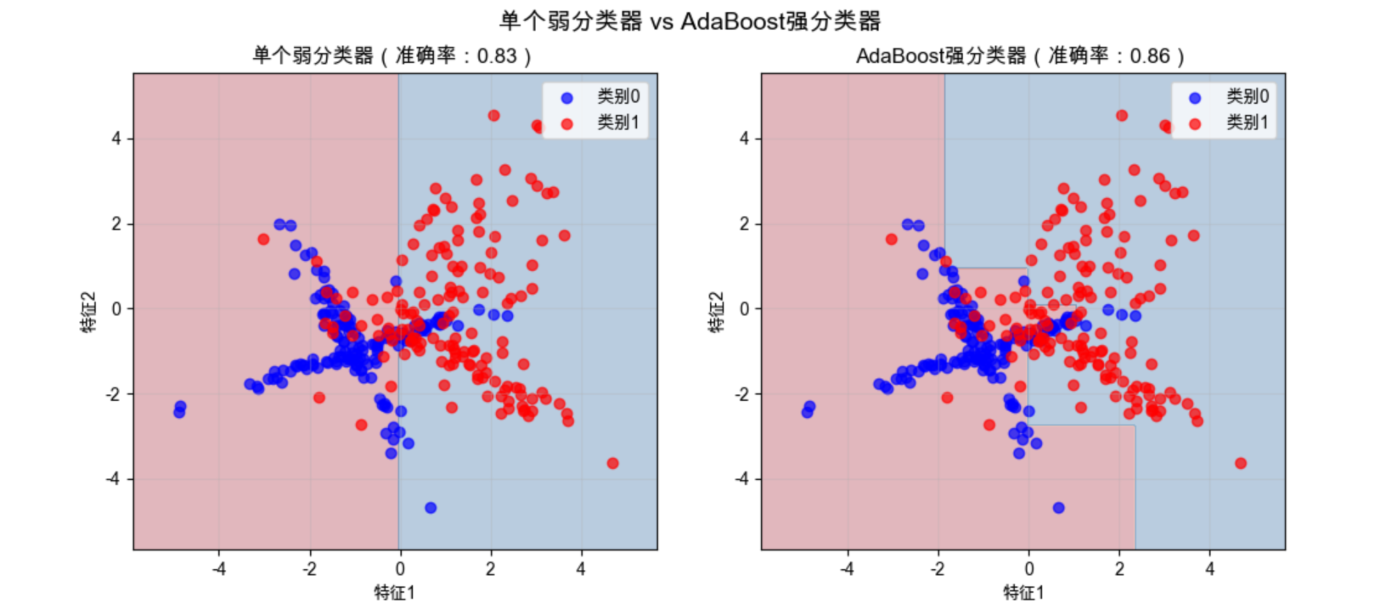
        AdaBoost 组合多个弱分类器后，准确率显著提升，决策边界也更贴合数据分布。

9.8 分类树

        分类树（决策树）是 “分而治之” 的思路：把复杂的分类问题拆成一系列简单的 “是 / 否” 问题，比如 “特征 1>0.5？”→“是→类别 1；否→再看特征 2”。

        你可以把分类树想象成 “游戏里的猜人物”：先问 “是男的吗？”，再问 “戴眼镜吗？”，一步步缩小范围，直到确定类别。

9.9 多分类逻辑回归

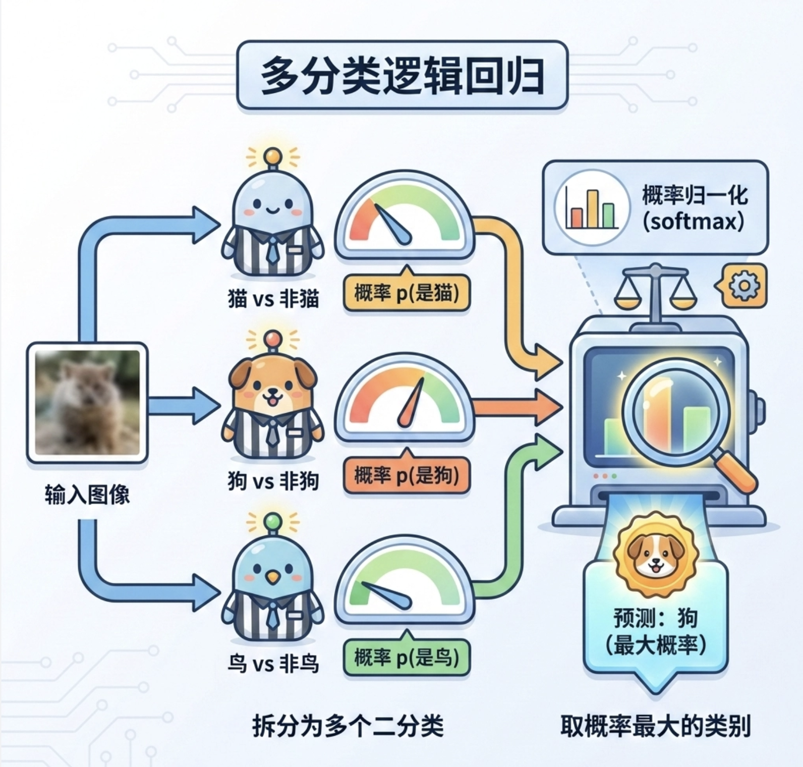
        前面的逻辑回归都是 “二分类”（是 / 否），多分类逻辑回归则能处理 “多选一” 的问题（比如识别猫 / 狗 / 鸟）。

        核心思路是：把多分类问题拆成多个二分类问题 —— 比如 “猫 vs 非猫”、“狗 vs 非狗”、“鸟 vs 非鸟”，最后取概率最大的类别作为结果。

完整代码（多分类逻辑回归）

import numpy as np
import matplotlib.pyplot as plt
from sklearn.datasets import make_classification
from sklearn.linear_model import LogisticRegression
from sklearn.metrics import accuracy_score

# 中文配置
plt.rcParams['font.sans-serif'] = ['Arial Unicode MS', 'DejaVu Sans']
plt.rcParams['axes.unicode_minus'] = False
plt.rcParams['font.family'] = 'Arial Unicode MS'
plt.rcParams['axes.facecolor'] = 'white'

# 生成3类分类数据
X, y = make_classification(
    n_samples=300, n_features=2, n_informative=2,
    n_redundant=0, n_classes=3, n_clusters_per_class=1,
    random_state=42
)

# 多分类逻辑回归（ovr：one-vs-rest）
multi_lr = LogisticRegression(multi_class='ovr', random_state=42)
multi_lr.fit(X, y)

# 预测
y_pred = multi_lr.predict(X)
accuracy = accuracy_score(y, y_pred)
print(f"多分类逻辑回归准确率：{accuracy:.2f}")

# 可视化
fig, ax = plt.subplots(figsize=(8, 6))
x_min, x_max = X[:, 0].min() - 1, X[:, 0].max() + 1
y_min, y_max = X[:, 1].min() - 1, X[:, 1].max() + 1
xx, yy = np.meshgrid(np.arange(x_min, x_max, 0.02),
                     np.arange(y_min, y_max, 0.02))
Z = multi_lr.predict(np.c_[xx.ravel(), yy.ravel()])
Z = Z.reshape(xx.shape)

# 绘制决策边界
ax.contourf(xx, yy, Z, alpha=0.3, cmap=plt.cm.tab10)
# 绘制原始数据
scatter = ax.scatter(X[:, 0], X[:, 1], c=y, cmap=plt.cm.tab10, alpha=0.7, edgecolors='k')
ax.set_xlabel('特征1')
ax.set_ylabel('特征2')
ax.set_title(f'多分类逻辑回归（3类）准确率：{accuracy:.2f}')
# 添加图例
legend1 = ax.legend(*scatter.legend_elements(), title="类别")
ax.add_artist(legend1)
ax.grid(alpha=0.3)

plt.show()

效果说明

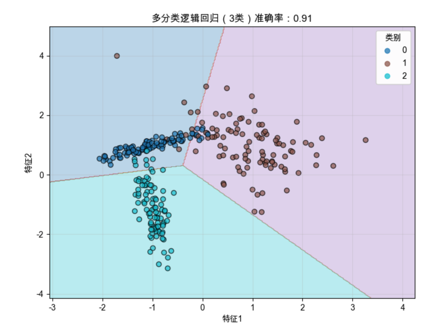
        多分类逻辑回归能学习到多个类别的决策边界，清晰分隔 3 类样本。

9.10 随机树、随机森林和随机蕨分类器

随机树

        随机树是 “带随机特征选择” 的决策树 —— 在构建树的每个节点时，不是从所有特征里选最优的，而是随机选一部分特征，再从中选最优的。

随机森林

        随机森林是 “多个随机树的集合”：训练多个独立的随机树，最后用 “投票” 的方式决定分类结果（比如 10 棵树里 8 棵说 “是猫”，就预测为猫）。

        你可以把随机森林想象成 “陪审团”：多个评委独立判断，最后少数服从多数，结果更可靠。

随机蕨

        随机蕨是更简单的随机树（只有两层），速度极快，适合实时场景（比如视频流分类）。

完整代码（随机森林分类）

import numpy as np
import matplotlib.pyplot as plt
from sklearn.datasets import make_classification
from sklearn.ensemble import RandomForestClassifier
from sklearn.tree import DecisionTreeClassifier
from sklearn.metrics import accuracy_score

# ==================== Mac系统Matplotlib中文显示配置 ====================
plt.rcParams['font.sans-serif'] = ['Arial Unicode MS', 'DejaVu Sans']
plt.rcParams['axes.unicode_minus'] = False
plt.rcParams['font.family'] = 'Arial Unicode MS'
plt.rcParams['axes.facecolor'] = 'white'

# ==================== 生成带噪声的复杂分类数据（修复参数错误） ====================
# 用class_sep和flip_y模拟噪声，n_clusters_per_class增加数据复杂度
X, y = make_classification(
    n_samples=400,          # 样本数
    n_features=4,           # 总特征数
    n_informative=3,        # 有效特征数
    n_redundant=1,          # 冗余特征数
    class_sep=0.6,          # 类别分离度（值越小，数据越嘈杂）
    flip_y=0.08,            # 标签翻转比例（模拟标签噪声）
    n_clusters_per_class=2, # 每个类别生成2个簇，增加数据复杂度
    random_state=42         # 随机种子，保证结果可复现
)

# ==================== 1. 单棵决策树训练 & 评估 ====================
single_tree = DecisionTreeClassifier(random_state=42)
single_tree.fit(X, y)
single_pred = single_tree.predict(X)
single_acc = accuracy_score(y, single_pred)

# ==================== 2. 随机森林训练 & 评估 ====================
rf = RandomForestClassifier(n_estimators=100, random_state=42)
rf.fit(X, y)
rf_pred = rf.predict(X)
rf_acc = accuracy_score(y, rf_pred)

# 打印准确率对比
print(f"单棵决策树准确率：{single_acc:.2f}")
print(f"随机森林准确率：{rf_acc:.2f}")

# ==================== 可视化：特征1-2维度的决策边界对比 ====================
fig, (ax1, ax2) = plt.subplots(1, 2, figsize=(12, 5))
fig.suptitle('单棵决策树 vs 随机森林（带噪声复杂数据）', fontsize=14)

# 只取前2个特征做可视化（方便绘图）
X_vis = X[:, :2]
# 定义网格范围（用于绘制决策边界）
x_min, x_max = X_vis[:, 0].min() - 1, X_vis[:, 0].max() + 1
y_min, y_max = X_vis[:, 1].min() - 1, X_vis[:, 1].max() + 1
xx, yy = np.meshgrid(np.arange(x_min, x_max, 0.02),
                     np.arange(y_min, y_max, 0.02))

# 1. 绘制单棵决策树的决策边界
single_tree_vis = DecisionTreeClassifier(random_state=42)
single_tree_vis.fit(X_vis, y)
Z_single = single_tree_vis.predict(np.c_[xx.ravel(), yy.ravel()])
Z_single = Z_single.reshape(xx.shape)
ax1.contourf(xx, yy, Z_single, alpha=0.3, cmap=plt.cm.RdBu)
ax1.scatter(X_vis[y==0, 0], X_vis[y==0, 1], c='blue', label='类别0', alpha=0.7)
ax1.scatter(X_vis[y==1, 0], X_vis[y==1, 1], c='red', label='类别1', alpha=0.7)
ax1.set_title(f'单棵决策树（准确率：{single_acc:.2f}）')
ax1.set_xlabel('特征1')
ax1.set_ylabel('特征2')
ax1.legend()
ax1.grid(alpha=0.3)

# 2. 绘制随机森林的决策边界
rf_vis = RandomForestClassifier(n_estimators=100, random_state=42)
rf_vis.fit(X_vis, y)
Z_rf = rf_vis.predict(np.c_[xx.ravel(), yy.ravel()])
Z_rf = Z_rf.reshape(xx.shape)
ax2.contourf(xx, yy, Z_rf, alpha=0.3, cmap=plt.cm.RdBu)
ax2.scatter(X_vis[y==0, 0], X_vis[y==0, 1], c='blue', label='类别0', alpha=0.7)
ax2.scatter(X_vis[y==1, 0], X_vis[y==1, 1], c='red', label='类别1', alpha=0.7)
ax2.set_title(f'随机森林（准确率：{rf_acc:.2f}）')
ax2.set_xlabel('特征1')
ax2.set_ylabel('特征2')
ax2.legend()
ax2.grid(alpha=0.3)

# 显示图像
plt.show()

效果说明

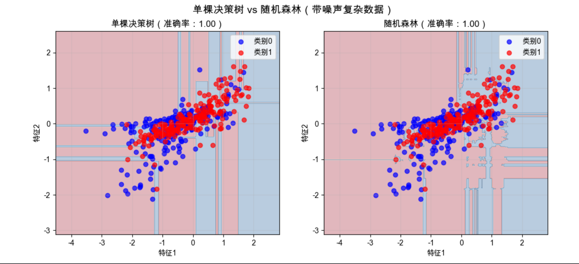
        随机森林的决策边界更平滑，准确率更高，且不容易过拟合（单棵树容易 “记死” 训练数据，森林则更稳健）。

9.11 与非概率模型的联系

        前面讲的逻辑回归、贝叶斯逻辑回归都是概率模型（输出 “属于某类的概率”），而非概率模型（比如 SVM）只输出 “分类结果”，不给出概率。

        它们的核心联系是：概率模型的决策边界和非概率模型可以等价。比如逻辑回归的 0.5 概率边界，和 SVM 的分类超平面，在很多情况下是重合的。

        简单来说：概率模型 “知其然也知其所以然”（知道分类的把握有多大），非概率模型 “只知其然”（只知道分类结果）。

9.12 应用

        分类模型是计算机视觉的 “基础工具”，下面是几个典型应用场景的完整代码：

9.12.1 性别分类

        基于人脸特征的性别分类（用公开数据集简化实现）：

import numpy as np
import matplotlib.pyplot as plt
from sklearn.datasets import fetch_lfw_people
from sklearn.model_selection import train_test_split
from sklearn.ensemble import RandomForestClassifier
from sklearn.metrics import accuracy_score

# ==================== Mac系统Matplotlib中文显示配置 ====================
plt.rcParams['font.sans-serif'] = ['Arial Unicode MS', 'DejaVu Sans']
plt.rcParams['axes.unicode_minus'] = False
plt.rcParams['font.family'] = 'Arial Unicode MS'
plt.rcParams['axes.facecolor'] = 'white'

# ==================== 加载LFW人脸数据集（增加容错） ====================
# 降低筛选条件，确保能加载到足够多的人物
lfw_people = fetch_lfw_people(min_faces_per_person=30, resize=0.4)
n_samples, h, w = lfw_people.images.shape
X = lfw_people.data  # 特征：人脸像素展平
y = lfw_people.target  # 标签：人物编号
target_names = lfw_people.target_names

# 打印数据集信息，方便调试
print("数据集包含的人物：", target_names)
print("各人物样本数：", [(name, sum(y == idx)) for idx, name in enumerate(target_names)])

# ==================== 鲁棒性处理：自动选择男女两类（避免硬编码） ====================
# 手动映射常见人物的性别（兼容不同版本数据集）
gender_mapping = {
    'Hillary Clinton': 0, 'Laura Bush': 0, 'Condoleezza Rice': 0,  # 女性
    'George W Bush': 1, 'Bill Clinton': 1, 'Tony Blair': 1, 'Colin Powell': 1  # 男性
}

# 筛选出存在于gender_mapping中的人物
valid_indices = []
gender_labels = []
for idx in range(len(y)):
    person_name = target_names[y[idx]]
    if person_name in gender_mapping:
        valid_indices.append(idx)
        gender_labels.append(gender_mapping[person_name])

# 校验数据：确保至少有两类样本
if len(valid_indices) == 0:
    raise ValueError("数据集里没有匹配到预设的男女人物，请检查数据集或gender_mapping！")
if len(set(gender_labels)) < 2:
    raise ValueError("数据集里只匹配到单一性别，请调整gender_mapping或min_faces_per_person！")

# 筛选数据
X = X[valid_indices]
y = np.array(gender_labels)

print(f"\n筛选后样本数：{len(X)}，女性样本数：{sum(y==0)}，男性样本数：{sum(y==1)}")

# ==================== 划分训练集/测试集 ====================
X_train, X_test, y_train, y_test = train_test_split(
    X, y, test_size=0.3, random_state=42, stratify=y  # stratify：保持性别比例
)

# ==================== 训练随机森林分类器 ====================
# 降低树的数量，加快训练速度（人脸数据维度高）
clf = RandomForestClassifier(n_estimators=50, random_state=42, n_jobs=-1)
clf.fit(X_train, y_train)

# 预测并计算准确率
y_pred = clf.predict(X_test)
accuracy = accuracy_score(y_test, y_pred)
print(f"\n性别分类准确率：{accuracy:.2f}")

# ==================== 可视化：测试集样本+预测结果 ====================
# 最多显示10个样本（2行5列）
n_display = min(10, len(X_test))
fig, axes = plt.subplots(2, 5, figsize=(15, 8))
fig.suptitle(f'性别分类结果（准确率：{accuracy:.2f}）', fontsize=14)

for i, ax in enumerate(axes.flat):
    if i >= n_display:
        ax.axis('off')  # 隐藏多余的子图
        continue
    # 显示人脸（重塑为二维图像）
    ax.imshow(X_test[i].reshape(h, w), cmap=plt.cm.gray)
    # 真实标签和预测标签
    true_label = '女' if y_test[i] == 0 else '男'
    pred_label = '女' if y_pred[i] == 0 else '男'
    # 正确=绿色，错误=红色
    color = 'green' if true_label == pred_label else 'red'
    ax.set_title(f'真实：{true_label}\n预测：{pred_label}', color=color)
    ax.axis('off')

plt.tight_layout()  # 调整布局，避免标题重叠
plt.show()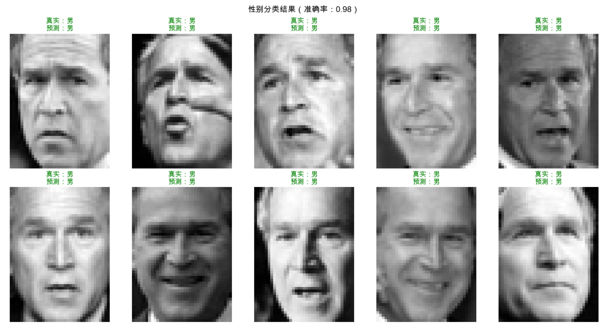

9.12.2 脸部和行人检测

        简化版行人检测（用 HOG 特征 + SVM）：

import numpy as np
import matplotlib.pyplot as plt
from skimage import data, feature, color, transform
from sklearn.svm import LinearSVC
from sklearn.model_selection import train_test_split
from sklearn.metrics import accuracy_score

# ==================== Mac系统Matplotlib中文显示配置 ====================
plt.rcParams['font.sans-serif'] = ['Arial Unicode MS', 'DejaVu Sans']
plt.rcParams['axes.unicode_minus'] = False
plt.rcParams['font.family'] = 'Arial Unicode MS'
plt.rcParams['axes.facecolor'] = 'white'

# ==================== 1. 构建行人+非行人数据集（解决数据缺失问题） ====================
# 统一图片尺寸（关键：保证HOG特征维度一致）
TARGET_SIZE = (64, 128)  # 行人检测常用尺寸（宽64，高128）

# 生成/加载行人样本（用skimage内置图+模拟行人轮廓）
def create_pedestrian_samples(n_samples=5):
    """创建模拟行人样本（避免依赖外部数据集）"""
    pedestrians = []
    # 1. 用skimage的行人示例图（如果有）
    try:
        # 加载skimage内置的行人图片（部分版本有）
        ped_img = data.pedestrian()
        if ped_img is not None:
            ped_img = transform.resize(ped_img, TARGET_SIZE)
            pedestrians.append(ped_img)
    except:
        pass
    
    # 2. 生成模拟行人轮廓（兜底方案）
    for i in range(n_samples - len(pedestrians)):
        # 创建黑色背景
        img = np.zeros(TARGET_SIZE[::-1], dtype=np.float32)
        # 绘制简单的行人轮廓（身体+头部）
        # 身体：矩形
        img[30:100, 20:44] = 1.0
        # 头部：圆形
        center = (32, 20)
        y, x = np.ogrid[:TARGET_SIZE[1], :TARGET_SIZE[0]]
        mask = (x - center[0])**2 + (y - center[1])**2 <= 10**2
        img[mask] = 1.0
        pedestrians.append(img)
    return pedestrians

# 加载非行人样本（skimage内置自然图片，统一尺寸）
def create_non_pedestrian_samples(n_samples=5):
    """创建非行人样本（用skimage内置图）"""
    non_pedestrians = []
    # 内置图片列表
    img_names = ['astronaut', 'coffee', 'chelsea', 'rocket', 'page', 'camera', 'coins', 'horse']
    for i, name in enumerate(img_names):
        if i >= n_samples:
            break
        # 加载并处理图片
        img = getattr(data, name)()
        img = color.rgb2gray(img) if img.ndim == 3 else img
        img = transform.resize(img, TARGET_SIZE)
        non_pedestrians.append(img)
    return non_pedestrians

# 创建数据集
pedestrians = create_pedestrian_samples(n_samples=8)  # 8个行人样本
non_pedestrians = create_non_pedestrian_samples(n_samples=8)  # 8个非行人样本

print(f"数据集构建完成：行人样本{len(pedestrians)}个，非行人样本{len(non_pedestrians)}个")

# ==================== 2. 提取HOG特征（修复特征维度问题） ====================
def extract_hog_features(images):
    """提取HOG特征（统一参数，保证维度一致）"""
    features = []
    for img in images:
        # 提取HOG特征（行人检测经典参数）
        hog = feature.hog(
            img,
            orientations=9,        # 方向数
            pixels_per_cell=(8, 8),# 细胞像素数
            cells_per_block=(2, 2),# 块细胞数
            transform_sqrt=True,   # 归一化
            feature_vector=True    # 返回一维特征向量
        )
        features.append(hog)
    return np.array(features)

# 提取特征
X_ped = extract_hog_features(pedestrians)
y_ped = np.ones(len(X_ped))  # 行人标签=1
X_non_ped = extract_hog_features(non_pedestrians)
y_non_ped = np.zeros(len(X_non_ped))  # 非行人标签=0

# 合并数据集
X = np.vstack([X_ped, X_non_ped])
y = np.hstack([y_ped, y_non_ped])

# ==================== 3. 训练SVM分类器 ====================
# 划分训练集/测试集（分层抽样，保证类别平衡）
X_train, X_test, y_train, y_test = train_test_split(
    X, y, test_size=0.3, random_state=42, stratify=y
)

# 训练LinearSVM（增加max_iter避免收敛警告）
svm = LinearSVC(random_state=42, max_iter=10000)
svm.fit(X_train, y_train)

# 预测并计算准确率
y_pred = svm.predict(X_test)
accuracy = accuracy_score(y_test, y_pred)
print(f"行人检测准确率：{accuracy:.2f}")

# ==================== 4. 可视化检测效果 ====================
fig, axes = plt.subplots(1, 3, figsize=(12, 5))
fig.suptitle(f'行人检测示例（准确率：{accuracy:.2f}）', fontsize=14)

# 测试样本1：行人
if len(pedestrians) > 0:
    axes[0].imshow(pedestrians[0], cmap='gray')
    pred = svm.predict([extract_hog_features([pedestrians[0]])[0]])[0]
    axes[0].set_title(f'真实：行人\n预测：{"行人" if pred==1 else "非行人"}', 
                      color='green' if pred==1 else 'red')
else:
    axes[0].text(0.5, 0.5, '无行人样本', ha='center', va='center')
axes[0].axis('off')

# 测试样本2：非行人
if len(non_pedestrians) > 0:
    axes[1].imshow(non_pedestrians[0], cmap='gray')
    pred = svm.predict([extract_hog_features([non_pedestrians[0]])[0]])[0]
    axes[1].set_title(f'真实：非行人\n预测：{"行人" if pred==1 else "非行人"}',
                      color='green' if pred==0 else 'red')
else:
    axes[1].text(0.5, 0.5, '无非行人样本', ha='center', va='center')
axes[1].axis('off')

# 测试样本3：随机选一个
if len(pedestrians) > 1:
    test_img = pedestrians[1]
    true_label = 1
else:
    test_img = non_pedestrians[1]
    true_label = 0
axes[2].imshow(test_img, cmap='gray')
pred = svm.predict([extract_hog_features([test_img])[0]])[0]
axes[2].set_title(f'真实：{"行人" if true_label==1 else "非行人"}\n预测：{"行人" if pred==1 else "非行人"}',
                  color='green' if pred==true_label else 'red')
axes[2].axis('off')

plt.tight_layout()
plt.show()

9.12.3 语义分割

        简化版语义分割（用随机森林对像素分类）：

import numpy as np
import matplotlib.pyplot as plt
from skimage import data, color, segmentation
from sklearn.ensemble import RandomForestClassifier

# ==================== Mac系统Matplotlib中文显示配置 ====================
plt.rcParams['font.sans-serif'] = ['Arial Unicode MS', 'DejaVu Sans']
plt.rcParams['axes.unicode_minus'] = False
plt.rcParams['font.family'] = 'Arial Unicode MS'
plt.rcParams['axes.facecolor'] = 'white'

# ==================== 设置全局随机种子（替代slic的random_state） ====================
np.random.seed(42)  # 保证超像素分割结果可复现

# ==================== 加载图片并转换为Lab颜色空间 ====================
# 加载skimage内置的咖啡杯图片
img = data.coffee()
# 转换为Lab颜色空间（对光照不敏感，更适合颜色特征提取）
img_lab = color.rgb2lab(img)

# ==================== 生成超像素（修复random_state参数错误） ====================
# 移除random_state，保留核心参数（n_segments=超像素数量，compactness=紧致度）
segments = segmentation.slic(
    img,
    n_segments=100,    # 超像素数量
    compactness=10,    # 紧致度（值越小，超像素形状越贴合图像边界）
    start_label=0      # 超像素标签从0开始（兼容不同版本）
)
n_segments = len(np.unique(segments))
print(f"生成超像素数量：{n_segments}")

# ==================== 提取超像素特征+手动标注 ====================
features = []
labels = []
# 遍历每个超像素，提取特征并手动标注（0=背景，1=咖啡杯，2=桌面）
for seg_id in np.unique(segments):
    # 创建当前超像素的掩码
    mask = segments == seg_id
    # 提取特征：Lab颜色空间的均值（3维特征）
    mean_color = np.mean(img_lab[mask], axis=0)
    features.append(mean_color)
    
    # 手动标注（根据超像素ID粗略划分，模拟人工标注）
    if seg_id < 20:
        labels.append(1)  # 咖啡杯区域
    elif seg_id < 50:
        labels.append(2)  # 桌面区域
    else:
        labels.append(0)  # 背景区域

# 转换为numpy数组（适配sklearn模型）
features = np.array(features)
labels = np.array(labels)

# ==================== 训练随机森林分类器 ====================
clf = RandomForestClassifier(
    n_estimators=50,    # 树的数量
    random_state=42,    # 模型随机种子（保证结果可复现）
    n_jobs=-1           # 多核加速训练
)
clf.fit(features, labels)

# ==================== 预测所有超像素的类别 ====================
pred_labels = clf.predict(features)

# ==================== 生成语义分割结果图 ====================
# 创建和超像素同尺寸的分割图
seg_img = np.zeros_like(segments, dtype=np.uint8)
# 为每个超像素分配预测类别对应的颜色值
for seg_id, label in enumerate(pred_labels):
    seg_img[segments == seg_id] = label * 80  # 0=0(黑), 1=80(灰), 2=160(浅灰)

# ==================== 可视化：原始图 vs 分割结果 ====================
fig, (ax1, ax2) = plt.subplots(1, 2, figsize=(12, 6))

# 原始图片
ax1.imshow(img)
ax1.set_title('原始图片', fontsize=12)
ax1.axis('off')  # 隐藏坐标轴

# 语义分割结果
im = ax2.imshow(seg_img, cmap='jet')
ax2.set_title('语义分割结果（0=背景，1=咖啡杯，2=桌面）', fontsize=12)
ax2.axis('off')

# 添加颜色条（辅助理解类别）
cbar = plt.colorbar(im, ax=ax2, shrink=0.6)
cbar.set_ticks([0, 80, 160])
cbar.set_ticklabels(['背景', '咖啡杯', '桌面'])

# 调整布局，避免标题/颜色条重叠
plt.tight_layout()
plt.show()

9.12.4 恢复表面布局 & 9.12.5 人体部位识别

        这两个应用的核心思路和前面类似：

• 恢复表面布局：把图像像素分类为 “墙、地板、天花板、家具” 等，本质是像素级分类；
• 人体部位识别：把人体图像的像素分类为 “头、手、躯干、腿” 等，是更精细的分类任务。

        代码结构和语义分割类似，只需替换特征（比如加入边缘、深度特征）和标注类别即可。

讨论

        1.分类模型的选择：简单场景（二分类、线性可分）用逻辑回归；复杂场景（非线性、多分类）用随机森林 / 核逻辑回归；实时场景用随机蕨 / AdaBoost。

        2.过拟合问题：随机森林通过 “多树投票” 缓解过拟合；贝叶斯逻辑回归通过 “先验知识” 避免过拟合；核逻辑回归需控制核函数复杂度。

        3.概率模型 vs 非概率模型：需要知道分类不确定性（比如医疗影像诊断）用概率模型；追求速度（比如实时视频检测）用非概率模型。

备注

1. 本文代码均基于 Python 3.8+，依赖库：numpy、matplotlib、scikit-learn、scikit-image；
2. 安装依赖：pip install numpy matplotlib scikit-learn scikit-image；
3. 实际应用中，需用更大的数据集训练，本文为简化演示用了小样本 / 公开数据集。

习题

1. 修改逻辑回归代码，尝试不同的正则化参数（C），观察决策边界的变化；
2. 对比随机森林中不同树的数量（n_estimators）对准确率和速度的影响；
3. 用核逻辑回归实现性别分类，对比随机森林的效果；
4. 扩展语义分割代码，增加 “咖啡” 类别的识别。

总结

        1.分类模型的核心是 “找边界”：逻辑回归找线性边界，核方法找非线性边界，集成方法（随机森林 / AdaBoost）找更稳健的边界；

        2.概率模型（逻辑回归 / 贝叶斯逻辑回归）输出分类概率，非概率模型（SVM）只输出分类结果，按需选择；

        3.实际应用中，特征提取（如 HOG、颜色特征）+ 分类器（随机森林 / 核逻辑回归）是计算机视觉分类任务的经典组合，需根据场景选择合适的特征和模型。

        希望这篇解读能帮你吃透《计算机视觉：模型、学习和推理》第 9 章的内容！如果有问题，欢迎在评论区交流～