可视化功能详解：如何看图与解读

一、数据分布可视化

1. 散点图（左侧）

图表外观与观察重点：
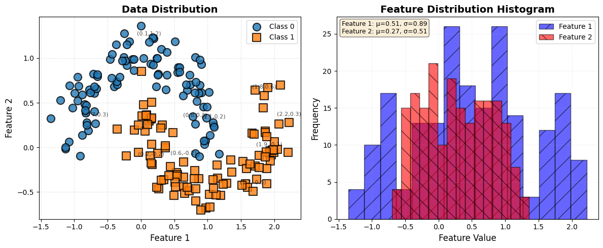
想象一个二维坐标系，横轴和纵轴通常代表数据的两个不同特征。图中有多组不同颜色（如蓝色、红色）的点集，每组代表一个数据类别。观察时重点看：不同颜色点的聚集位置、组与组之间的分离程度、点的分布密度，以及是否有明显偏离群体的异常点。

核心解读意义：
散点图是数据探索的第一步，它直观地揭示了数据的“天生”结构。

1. 可分离性判断：这是最重要的一点。它能直接告诉你手头是一个“简单”问题还是“复杂”问题。如果不同颜色的点群各自成团，中间有清晰的空白地带，说明数据可能是线性或近似线性可分的，简单的模型（如逻辑回归、线性SVM）就可能取得好效果。如果点群相互纠缠、犬牙交错，则意味着这是一个非线性可分问题，需要更强大的模型（如带核函数的SVM、神经网络）来捕捉复杂的决策边界。
2. 数据关系洞察：观察点的分布趋势。是呈现线性带状、曲线簇状还是无规则的云团状？这能启发你对特征间关系的理解，例如是否可以考虑特征交叉项或多项式特征。
3. 异常值检测：远离主体点群的孤立点很可能是异常值或噪声。这些点会对模型的训练产生不成比例的影响，尤其是对距离敏感的模型（如KNN、SVM），需要在预处理阶段予以关注。
4. 类别平衡评估：粗略对比不同颜色点的数量，可以初步判断数据集是否平衡。严重的类别不平衡会影响许多模型的训练，可能需要重采样策略。

思考与行动建议：

• “看图后问自己：两类数据是‘楚河汉界’还是‘你中有我’？”
• 如果分离清晰：可以优先尝试简单、可解释性强的线性模型。
• 如果混杂严重：需要准备使用非线性模型，并考虑是否需要更多的特征工程（如特征变换）或更多数据。
• 如果存在异常点：需要检查数据来源，决定是剔除、修正还是采用鲁棒性更强的模型。

---

2. 特征分布直方图（右侧）

图表外观与观察重点：
这是一个并排或叠加的柱状图，横轴是特征值（被分成了多个小区间），纵轴是该区间内样本出现的频次。通常会为不同的特征（如特征1和特征2）绘制不同颜色、半透明的直方图以方便对比。

核心解读意义：
直方图展示了单个特征的“统计学肖像”，是进行数据预处理的重要依据。

1. 尺度与范围：不同特征的取值区间可能差异巨大。例如，特征1的值在 [0, 1] 之间，而特征2在 [0, 10000] 之间。对于基于梯度下降的模型（如神经网络、逻辑回归），这种尺度差异会导致优化困难，使训练过程缓慢或不稳定。此时，特征标准化（如Z-score）或归一化（缩放到[0,1]）是必要的。
2. 分布形态：观察分布是接近对称的“钟形”（正态分布）、偏向一边（偏态分布），还是存在多个峰值（多峰分布）？许多模型（如线性回归、高斯朴素贝叶斯）隐含着数据服从正态分布的假设。严重的偏态可能需要通过对数变换、平方根变换等进行校正。
3. 特征间对比：比较不同特征的分布形状和集中趋势。如果两个特征分布形态相似且尺度接近，说明它们可能受相似因素影响，或者其中一个可能是冗余的。
4. 异常值再确认：直方图的长尾部分（远离主峰的孤立小柱）可以再次佐证散点图中发现的异常值。

思考与行动建议：

• “看图后问自己：我的各个特征是在同一个‘量级擂台’上比武吗？”
• 如果尺度差异大：必须进行特征缩放（Scaling）。
• 如果分布严重偏斜：考虑进行数据变换，使其更接近正态分布。
• 如果存在极端长尾/异常值：需要决定处理策略，如缩尾处理（Winsorizing）。

---

示例代码

1. Scatter Plot (Left)

def plot_enhanced_data_distribution(x_data, y_data, title="Data Distribution"):
    """
    Enhanced scatter plot with better color differentiation
    """
    plt.figure(figsize=(12, 5))
    
    # Left: Scatter plot
    plt.subplot(1, 2, 1)
    
    # Use distinct colors with different markers
    colors = ['#1f77b4', '#ff7f0e']  # Blue and orange
    markers = ['o', 's']  # Circle and square
    sizes = [120, 120]  # Marker sizes
    edge_colors = ['black', 'black']  # Black borders
    
    for i in range(2):
        mask = (y_data == i)
        plt.scatter(x_data[mask, 0].numpy(), 
                   x_data[mask, 1].numpy(),
                   c=colors[i], 
                   marker=markers[i],
                   s=sizes[i],
                   edgecolor=edge_colors[i],
                   linewidth=1.5,
                   alpha=0.8,
                   label=f'Class {i}')
    
    plt.xlabel('Feature 1', fontsize=12)
    plt.ylabel('Feature 2', fontsize=12)
    plt.title(title, fontsize=14, fontweight='bold')
    plt.legend(fontsize=10, loc='best')
    plt.grid(True, alpha=0.3, linestyle='--')
    
    # Add value annotations for key points
    for idx, (x, y) in enumerate(zip(x_data[:, 0], x_data[:, 1])):
        plt.annotate(f'({x:.1f},{y:.1f})', 
                    (x, y),
                    textcoords="offset points",
                    xytext=(0, 10),
                    ha='center',
                    fontsize=8,
                    alpha=0.7)
    
    # Right: Feature distribution histogram
    plt.subplot(1, 2, 2)
    
    # Plot histograms with different styles
    n_bins = 15
    plt.hist(x_data[:, 0].numpy(), 
             bins=n_bins, 
             alpha=0.6, 
             color='blue',
             edgecolor='black',
             linewidth=1,
             label='Feature 1',
             hatch='/')
    
    plt.hist(x_data[:, 1].numpy(), 
             bins=n_bins, 
             alpha=0.6, 
             color='red',
             edgecolor='black',
             linewidth=1,
             label='Feature 2',
             hatch='\\')
    
    plt.xlabel('Feature Value', fontsize=12)
    plt.ylabel('Frequency', fontsize=12)
    plt.title('Feature Distribution Histogram', fontsize=14, fontweight='bold')
    plt.legend(fontsize=10)
    plt.grid(True, alpha=0.3, linestyle=':')
    
    # Add statistics text
    stats_text = f'Feature 1: μ={x_data[:,0].mean():.2f}, σ={x_data[:,0].std():.2f}\n'
    stats_text += f'Feature 2: μ={x_data[:,1].mean():.2f}, σ={x_data[:,1].std():.2f}'
    plt.text(0.02, 0.98, stats_text,
             transform=plt.gca().transAxes,
             fontsize=9,
             verticalalignment='top',
             bbox=dict(boxstyle='round', facecolor='wheat', alpha=0.5))
    
    plt.tight_layout()
    plt.show()

Key Design Principles:

Color Scheme: Use matplotlib's default color cycle for consistency

Marker Differentiation: Different shapes for different classes

Edge Colors: Black borders for clear separation

Annotations: Show coordinate values for clarity

Statistics: Include mean and std in text box

二、训练过程监控图

1. 损失曲线图（左侧）

图表外观与观察重点：
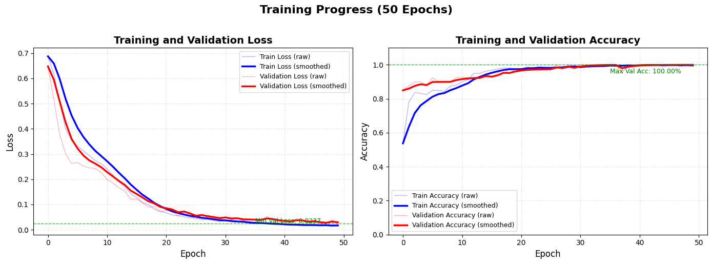
这是一条或两条随着训练轮次（Epoch）增加而变化的曲线。横轴是Epoch，纵轴是损失值（Loss）。通常包含“训练损失”曲线，在完整训练集中还可能包含“验证损失”曲线。损失值越低越好。

核心解读意义：
损失曲线是模型训练的“心电图”，直接反映了优化算法的工作状态和学习进度。

1. 收敛性诊断：理想的曲线应在初期快速下降，随后下降速度放缓，最终在一个小范围内平稳波动或几乎不再下降，这代表模型已经收敛到了一个（局部）最优点。
2. 过拟合/欠拟合识别：这是其核心价值。
   • 健康状态：训练损失和验证损失同步下降，最终两者都保持较低水平且差距很小。
   • 过拟合警报：训练损失持续下降，但验证损失在某个点后开始持续上升。这表明模型开始“死记硬背”训练数据的细节（包括噪声），而丧失了泛化到新数据的能力。这是需要立即干预的信号（如早停）。
   • 欠拟合迹象：两条曲线都下降得非常缓慢，甚至在很多轮次后仍处于很高的平台。这表明模型能力不足（太简单）或训练配置有问题（如学习率太低），无法有效捕捉数据中的模式。
3. 学习率调优参考：曲线下降的形态能反映学习率设置是否合适。
   • 学习率恰当时：曲线平滑稳定下降。
   • 学习率太大时：曲线可能剧烈震荡，损失值上下跳动，无法稳定收敛。
   • 学习率太小时：曲线下降得像蜗牛爬行，需要极多的训练轮次才能收敛。

思考与行动建议：

• “看图后问自己：模型是‘学得好’、‘学过头了’还是‘没学会’？”
• 见过拟合：实施正则化（L1/L2、Dropout）、获取更多数据、使用数据增强、或采用早停策略。
• 见欠拟合：尝试更复杂的模型、增加训练轮次、检查特征有效性、或适当提高学习率。
• 见震荡：降低学习率，或使用带有动量（Momentum）或自适应学习率（如Adam）的优化器。

2. 准确率曲线图（右侧）

图表外观与观察重点：
与损失曲线类似，横轴是Epoch，纵轴是准确率（或其他评估指标，如F1-score），范围通常在0%到100%之间。同样包含“训练准确率”和“验证准确率”曲线。准确率越高越好。

核心解读意义：
准确率曲线是模型性能的“成绩单”，从最终任务目标的角度评估训练效果。

1. 性能天花板评估：曲线最终稳定在的水平，代表了当前模型架构和数据集下可能达到的最佳性能。如果这个值远低于业务要求，可能需要从根本上调整模型或获取更有区分度的特征。
2. 过拟合/欠拟合的另一个视角：
   • 健康状态：两条准确率曲线共同上升，最终都达到较高值且差距不大。
   • 过拟合：训练准确率可能接近100%，但验证准确率显著较低，且差距随着训练拉大。
   • 欠拟合：两条曲线都很低，且提升缓慢。
3. 训练稳定性观察：曲线是否平滑上升，是否存在剧烈的“锯齿状”波动？波动可能意味着批次大小（Batch Size）设置过小，或学习率过高。

思考与行动建议：

• “看图后问自己：模型最终‘考了多少分’？这个分数稳定吗？”
• 性能天花板低：考虑更复杂的模型、深入的特征工程或检查数据标签质量。
• 训练/验证差距大（过拟合）：同损失曲线的建议，侧重于提升泛化能力。
• 曲线波动大：尝试增大Batch Size，或使用学习率衰减策略。

---

示例代码

2. Loss and Accuracy Curves - Clean Version

def plot_training_curves_clean(train_losses, val_losses, 
                              train_accuracies, val_accuracies,
                              smoothing_factor=0.6):
    """
    Clean and professional training curves with smoothing
    """
    fig, axes = plt.subplots(1, 2, figsize=(14, 5))
    
    # Apply exponential smoothing for better visualization
    def smooth_curve(data, factor=0.6):
        smoothed = []
        for i in range(len(data)):
            if i == 0:
                smoothed.append(data[i])
            else:
                smoothed.append(factor * smoothed[-1] + (1 - factor) * data[i])
        return smoothed
    
    smooth_train_loss = smooth_curve(train_losses, smoothing_factor)
    smooth_val_loss = smooth_curve(val_losses, smoothing_factor)
    smooth_train_acc = smooth_curve(train_accuracies, smoothing_factor)
    smooth_val_acc = smooth_curve(val_accuracies, smoothing_factor)
    
    # 1. Loss Curves Plot
    axes[0].plot(train_losses, 
                 color='blue', 
                 alpha=0.3,
                 linewidth=1,
                 label='Train Loss (raw)')
    
    axes[0].plot(smooth_train_loss, 
                 color='blue', 
                 linewidth=2.5,
                 label='Train Loss (smoothed)')
    
    axes[0].plot(val_losses, 
                 color='red', 
                 alpha=0.3,
                 linewidth=1,
                 label='Validation Loss (raw)')
    
    axes[0].plot(smooth_val_loss, 
                 color='red', 
                 linewidth=2.5,
                 label='Validation Loss (smoothed)')
    
    axes[0].set_xlabel('Epoch', fontsize=12)
    axes[0].set_ylabel('Loss', fontsize=12)
    axes[0].set_title('Training and Validation Loss', 
                     fontsize=14, fontweight='bold')
    axes[0].legend(fontsize=9, loc='best')
    axes[0].grid(True, alpha=0.3, linestyle='--')
    
    # Set y-axis to log scale if losses vary widely
    if max(train_losses) / min(train_losses[train_losses > 0]) > 100:
        axes[0].set_yscale('log')
    
    # Add horizontal line at min validation loss
    min_val_loss_idx = np.argmin(val_losses)
    axes[0].axhline(y=val_losses[min_val_loss_idx], 
                   color='green', 
                   linestyle='--',
                   alpha=0.7,
                   linewidth=1)
    axes[0].text(len(val_losses)*0.7, val_losses[min_val_loss_idx]*1.1,
                f'Min Val Loss: {val_losses[min_val_loss_idx]:.4f}',
                fontsize=9, color='green')
    
    # 2. Accuracy Curves Plot
    axes[1].plot(train_accuracies, 
                 color='blue', 
                 alpha=0.3,
                 linewidth=1,
                 label='Train Accuracy (raw)')
    
    axes[1].plot(smooth_train_acc, 
                 color='blue', 
                 linewidth=2.5,
                 label='Train Accuracy (smoothed)')
    
    axes[1].plot(val_accuracies, 
                 color='red', 
                 alpha=0.3,
                 linewidth=1,
                 label='Validation Accuracy (raw)')
    
    axes[1].plot(smooth_val_acc, 
                 color='red', 
                 linewidth=2.5,
                 label='Validation Accuracy (smoothed)')
    
    axes[1].set_xlabel('Epoch', fontsize=12)
    axes[1].set_ylabel('Accuracy', fontsize=12)
    axes[1].set_title('Training and Validation Accuracy', 
                     fontsize=14, fontweight='bold')
    axes[1].legend(fontsize=9, loc='best')
    axes[1].grid(True, alpha=0.3, linestyle='--')
    
    # Set y-axis limits for accuracy (0-100%)
    axes[1].set_ylim([0, 1.1])
    
    # Add horizontal line at max validation accuracy
    max_val_acc_idx = np.argmax(val_accuracies)
    axes[1].axhline(y=val_accuracies[max_val_acc_idx], 
                   color='green', 
                   linestyle='--',
                   alpha=0.7,
                   linewidth=1)
    axes[1].text(len(val_accuracies)*0.7, val_accuracies[max_val_acc_idx]*0.95,
                f'Max Val Acc: {val_accuracies[max_val_acc_idx]:.2%}',
                fontsize=9, color='green')
    
    # Add epoch information
    fig.suptitle(f'Training Progress ({len(train_losses)} Epochs)', 
                fontsize=16, fontweight='bold', y=1.02)
    
    plt.tight_layout()
    plt.show()

Key Design Principles:

Dual Lines: Show both raw (thin, transparent) and smoothed (thick, opaque) curves

Clear Color Coding: Blue for training, Red for validation

Reference Lines: Highlight minimum loss and maximum accuracy

Log Scale: Automatically use log scale for wide-ranging losses

Grid Lines: Dashed grid for better readability

三、决策边界可视化

图表外观与观察重点：
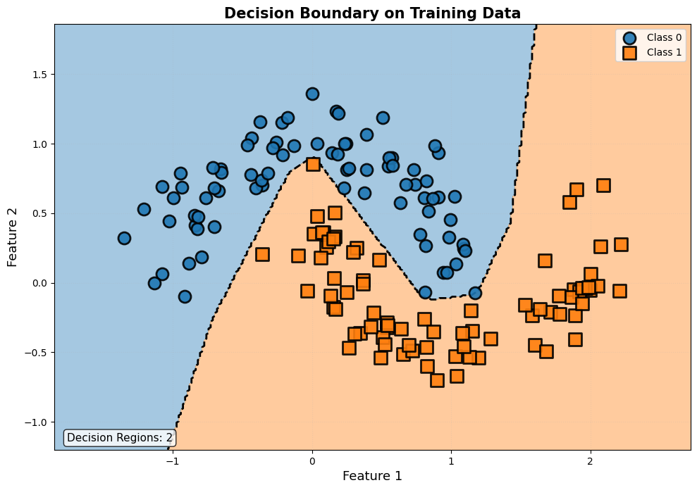
这是一张背景被不同颜色（如浅蓝和浅红）区域填充的图，代表了模型对二维平面上每一个点的分类预测。原始的散点数据（带颜色的实心点）会叠加在上面。观察重点是背景色区域的分界线（决策边界）的形状，以及原始数据点相对于这条边界的位置。

核心解读意义：
决策边界图将模型的“思考过程”和“判断标准”进行了前所未有的可视化，是理解模型行为的关键。

1. 模型复杂度的直观体现：
   • 平滑的直线或曲线：通常代表一个泛化能力较好的模型，它学到了数据背后的主要规律。
   • 极其弯曲、迂回、充满“锯齿”或小洞的边界：这是典型的过拟合迹象。模型为了完美分类每一个训练点（包括噪声），构造了极其复杂的规则，这种规则在新数据上会很差。
2. 分类正确性的空间检查：你可以一目了然地看到是否有某个颜色的点落在了相反颜色的背景区域里，这些点就是被模型分错的样本。观察这些错误点是在边界附近（情有可原），还是远离边界（模型可能对某类特征有系统性误解）。
3. 模型类型验证：它验证了你所使用的模型是否如预期般工作。例如，线性模型应该产生直线边界，多项式核SVM会产生平滑曲线，而决策树或最近邻类模型则容易产生不规则的阶梯状或细胞状边界。

思考与行动建议：

• “看图后问自己：模型的‘判案规则’是清晰合理的法令，还是针对每个案例的特殊条款？”
• 边界过于复杂：这是最强的过拟合视觉信号。必须增加正则化强度、简化模型，或收集更多数据。
• 存在系统性误分类区域：检查该区域样本的特征，可能是特征工程不充分，未能提供足够的区分信息。
• 边界过于简单，错误点很多：模型可能欠拟合，需要增加其复杂度。

---

示例代码

3. Decision Boundary with Clear Separation

def plot_decision_boundary_clear(model, x_data, y_data, title="Decision Boundary"):
    """
    Clear decision boundary visualization with proper styling
    """
    # Create mesh grid
    x_min, x_max = x_data[:, 0].min() - 0.5, x_data[:, 0].max() + 0.5
    y_min, y_max = x_data[:, 1].min() - 0.5, x_data[:, 1].max() + 0.5
    
    xx, yy = np.meshgrid(np.linspace(x_min, x_max, 300),
                         np.linspace(y_min, y_max, 300))
    
    # Get predictions
    model.eval()
    with torch.no_grad():
        grid_tensor = torch.FloatTensor(np.c_[xx.ravel(), yy.ravel()])
        logits = model(grid_tensor)
        predictions = torch.argmax(logits, dim=1)
        Z = predictions.numpy().reshape(xx.shape)
    
    # Create figure
    plt.figure(figsize=(10, 8))
    
    # Create custom colormap for clear separation
    from matplotlib.colors import ListedColormap
    colors = ['#1f77b4', '#ff7f0e']  # Blue and orange
    cmap = ListedColormap(colors)
    
    # Plot decision boundary with contour lines
    plt.contourf(xx, yy, Z, 
                 alpha=0.4, 
                 cmap=cmap,
                 levels=[-0.5, 0.5, 1.5])
    
    # Add contour lines for boundary
    contour = plt.contour(xx, yy, Z, 
                         levels=[0.5], 
                         colors='black',
                         linewidths=2,
                         linestyles='dashed')
    
    # Plot training data points with enhanced styling
    markers = ['o', 's']  # Circle and square
    sizes = [150, 150]  # Large markers
    edge_colors = ['black', 'black']
    linewidths = [2, 2]
    
    for i in range(2):
        mask = (y_data == i)
        plt.scatter(x_data[mask, 0].numpy(), 
                   x_data[mask, 1].numpy(),
                   c=colors[i],
                   marker=markers[i],
                   s=sizes[i],
                   edgecolor=edge_colors[i],
                   linewidth=linewidths[i],
                   alpha=0.9,
                   label=f'Class {i} (Train)',
                   zorder=5)  # Bring points to front
    
    # Add test data if available (different markers)
    if 'x_test' in locals():
        for i in range(2):
            mask = (y_test == i)
            plt.scatter(x_test[mask, 0].numpy(),
                       x_test[mask, 1].numpy(),
                       c=colors[i],
                       marker='*' if i == 0 else 'D',  # Star and diamond
                       s=200,
                       edgecolor='black',
                       linewidth=2,
                       alpha=1.0,
                       label=f'Class {i} (Test)',
                       zorder=6)  # Bring test points to very front
    
    # Plot parameters
    plt.xlabel('Feature 1', fontsize=13)
    plt.ylabel('Feature 2', fontsize=13)
    plt.title(title, fontsize=15, fontweight='bold')
    plt.legend(fontsize=10, loc='best')
    plt.grid(True, alpha=0.2, linestyle=':')
    
    # Add boundary information
    plt.text(0.02, 0.02, 
            f'Decision Regions: {np.unique(Z).size}',
            transform=plt.gca().transAxes,
            fontsize=11,
            bbox=dict(boxstyle='round', facecolor='white', alpha=0.8))
    
    # Set aspect ratio to equal for proper visualization
    plt.gca().set_aspect('equal', adjustable='box')
    
    plt.tight_layout()
    plt.show()

Key Design Principles:

High-Resolution Grid: 300×300 grid for smooth boundaries

Custom Colormap: Distinct colors for each class

Boundary Lines: Dashed black line showing exact decision boundary

Layered Plotting: Points on top of background, test points on very top

Different Markers: Distinct shapes for training vs test data

四、Confusion Matrix Visualization

四、混淆矩阵

图表外观与观察重点：
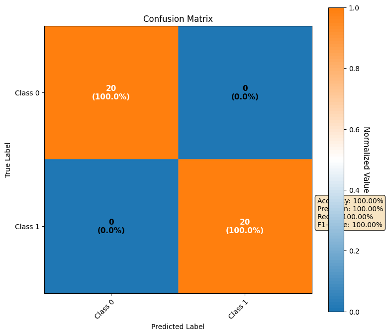
一个N×N的方格矩阵（N为类别数），通常以热力图形式呈现，颜色深浅代表数值大小。矩阵的行代表样本的真实标签，列代表模型的预测标签。对角线上的格子（第i行第i列）表示被正确分类的样本数，其他格子则表示各种类型的分类错误。

核心解读意义：
混淆矩阵超越了单一的准确率，揭示了模型错误的详细构成，对于多分类问题和不平衡数据集尤为重要。

1. 错误类型剖析：它清晰地告诉你模型具体“错在了哪里”。例如，是将A类误判为B类多，还是将B类误判为A类多？这在实际业务中代价可能完全不同（如疾病诊断中，假阴性和假阳性的后果差异巨大）。
2. 模型偏好的诊断：在不平衡数据集中，一个追求高准确率的模型可能会倾向于将所有样本都预测为多数类。这在混淆矩阵中表现为：多数类所在行/列的对角线值很高，但少数类所在行/列的值几乎全部分布在错误格子里。
3. 关键指标的计算基础：精确率（Precision）、召回率（Recall）、F1分数等更细致的指标，都可以直接从混淆矩阵中计算得出。例如，对于“猫”这个类别，其精确率 = （预测为猫且正确的数量）/（所有被预测为猫的数量），召回率 = （预测为猫且正确的数量）/（真实为猫的总数量）。

思考与行动建议：

• “看图后问自己：模型的错误是‘随机失误’还是‘系统性偏见’？”
• 发现特定类别混淆：例如，模型总是分不清“猫”和“狗”。这说明这两个类的特征可能非常相似，需要针对性地增加能区分它们的特征，或收集更多这两类的困难样本进行训练。
• 发现模型偏向多数类：需要使用适用于不平衡数据的策略，如对少数类进行上采样、对多数类进行下采样、在损失函数中使用类别权重（Class Weight）等。
• 根据不同错误成本调整：如果混淆矩阵显示某种错误（如假阴性）代价很高，你可以通过调整分类阈值（Threshold）来优化模型，提高召回率（尽管可能会降低精确率）。

---

示例代码

4. Professional Confusion Matrix Heatmap

def plot_confusion_matrix_professional(cm, class_names=None, title="Confusion Matrix"):
    """
    Professional confusion matrix visualization
    """
    if class_names is None:
        class_names = [f'Class {i}' for i in range(len(cm))]
    
    fig, ax = plt.subplots(figsize=(8, 7))
    
    # Normalize the confusion matrix for better color scaling
    cm_normalized = cm.astype('float') / cm.sum(axis=1)[:, np.newaxis]
    
    # Create custom colormap
    import seaborn as sns
    from matplotlib.colors import LinearSegmentedColormap
    
    # Blue to white to red colormap
    colors = ["#1f77b4", "white", "#ff7f0e"]
    n_bins = 100
    cmap = LinearSegmentedColormap.from_list("custom_div", colors, N=n_bins)
    
    # Plot heatmap
    im = ax.imshow(cm_normalized, interpolation='nearest', cmap=cmap)
    
    # Create colorbar
    cbar = ax.figure.colorbar(im, ax=ax)
    cbar.ax.set_ylabel('Normalized Value', rotation=-90, va="bottom", fontsize=11)
    
    # Set labels
    ax.set(xticks=np.arange(cm.shape[1]),
           yticks=np.arange(cm.shape[0]),
           xticklabels=class_names,
           yticklabels=class_names,
           title=title,
           ylabel='True Label',
           xlabel='Predicted Label')
    
    # Rotate tick labels
    plt.setp(ax.get_xticklabels(), rotation=45, ha="right", rotation_mode="anchor")
    
    # Add text annotations
    thresh = cm_normalized.max() / 2.
    for i in range(cm.shape[0]):
        for j in range(cm.shape[1]):
            # Show both raw count and percentage
            text = f'{cm[i, j]}\n({cm_normalized[i, j]:.1%})'
            color = "white" if cm_normalized[i, j] > thresh else "black"
            ax.text(j, i, text,
                   ha="center", va="center",
                   color=color,
                   fontsize=11,
                   fontweight='bold')
    
    # Add performance metrics
    accuracy = np.trace(cm) / np.sum(cm)
    metrics_text = f'Accuracy: {accuracy:.2%}'
    
    # Calculate additional metrics for binary classification
    if len(cm) == 2:
        TP, FN, FP, TN = cm[1, 1], cm[1, 0], cm[0, 1], cm[0, 0]
        precision = TP / (TP + FP) if (TP + FP) > 0 else 0
        recall = TP / (TP + FN) if (TP + FN) > 0 else 0
        f1 = 2 * (precision * recall) / (precision + recall) if (precision + recall) > 0 else 0
        
        metrics_text += f'\nPrecision: {precision:.2%}\nRecall: {recall:.2%}\nF1-Score: {f1:.2%}'
    
    plt.text(1.02, 0.3, metrics_text,
             transform=ax.transAxes,
             fontsize=10,
             verticalalignment='center',
             bbox=dict(boxstyle='round', facecolor='wheat', alpha=0.8))
    
    # Add grid lines
    ax.set_xticks(np.arange(cm.shape[1]+1)-0.5, minor=True)
    ax.set_yticks(np.arange(cm.shape[0]+1)-0.5, minor=True)
    ax.grid(which="minor", color="gray", linestyle='-', linewidth=0.5)
    ax.tick_params(which="minor", size=0)
    
    fig.tight_layout()
    plt.show()
    
    return fig, ax

Key Design Principles:

Dual Annotation: Shows both count and percentage in each cell

Custom Colormap: Diverging colormap (blue-white-orange) for clear contrast

Smart Text Colors: White text on dark cells, black text on light cells

Performance Metrics: Automatic calculation and display of metrics

Grid Lines: Subtle grid for cell separation

五、综合解读与行动指南

如何讲一个完整的“训练故事”：

结合所有图表，你可以像叙述一个故事一样描述训练过程：
“初期（Epoch 1-5）：损失曲线陡降，准确率快速攀升，决策边界从一条随机线迅速移动到一个大致合理的位置，说明模型正在快速学习基础模式。
中期（Epoch 6-20）：损失下降放缓，准确率缓慢提升至90%以上，决策边界变得越发精细和平滑，验证曲线与训练曲线保持良好同步，这是健康的优化阶段。
后期（Epoch 21-50）：训练损失降至接近零，训练准确率达100%，但验证损失停止下降并开始轻微上扬，验证准确率在95%处徘徊。决策边界出现轻微的不必要弯曲以‘包裹’个别训练点。综合判断：模型开始出现过拟合迹象。
决策：采用‘早停’策略，回退到第20个Epoch的模型权重，该状态是验证集上表现最好的。”

模型质量快速诊断清单：

观察点	健康迹象	问题迹象	可能原因与行动
损失曲线	双线平稳下降，收敛后差距小	验证损失上升；双线居高不下	过拟合：早停、正则化、更多数据。 欠拟合：增加模型复杂度、调大学习率、检查特征。
准确率曲线	双线同步上升至高值，差距小	验证准确率远低于训练；双线都很低	过拟合：同上。 欠拟合/模型能力不足：换更强模型、特征工程。
决策边界	平滑，与数据点群间隔合理	极不规则，为拟合每个点弯曲	严重过拟合：加强正则化、简化模型。
混淆矩阵	对角线颜色深，其他格子颜色浅	非对角线有深色块；某一行/列几乎全错	类别混淆/不平衡：针对性增加特征、调整类别权重、重采样。

实用调试流程建议：

1. 第一看：数据本身（散点图/直方图）。确保数据是“可学的”且特征是“准备好的”。如果数据一团糟，模型再强也无用。
2. 第二看：学习过程（损失/准确率曲线）。判断训练是否正常，是欠拟合还是过拟合，并据此调整模型容量、正则化和学习率。
3. 第三看：模型行为（决策边界）。直观感受模型的判断逻辑是否合理，确认过拟合/欠拟合的视觉证据。
4. 第四看：性能细节（混淆矩阵）。深入分析错误类型，针对性地改进模型或调整决策阈值以满足业务需求。

通过系统性地观察和解读这些可视化图表，你将能够超越黑箱调参，真正理解你的模型，并做出明智、高效的改进决策。可视化不仅是展示结果的工具，更是驱动模型迭代开发的指南针。

完整可运行展示代码

import torch
import torch.nn as nn
import torch.optim as optim
import numpy as np
import matplotlib.pyplot as plt
from sklearn.datasets import make_moons, make_classification
from sklearn.model_selection import train_test_split
from sklearn.metrics import confusion_matrix
import seaborn as sns
from matplotlib.colors import LinearSegmentedColormap, ListedColormap

# 设置中文字体（如果需要）
# plt.rcParams['font.sans-serif'] = ['SimHei']
# plt.rcParams['axes.unicode_minus'] = False

# ========== 1. 数据生成 ==========
def generate_data(n_samples=200, noise=0.1, random_state=42):
    """生成示例数据"""
    # 使用make_moons创建非线性可分数据
    X, y = make_moons(n_samples=n_samples, noise=noise, random_state=random_state)
    
    # 转换为PyTorch张量
    X_tensor = torch.FloatTensor(X)
    y_tensor = torch.LongTensor(y)
    
    return X_tensor, y_tensor

# ========== 2. 简单神经网络模型 ==========
class SimpleNN(nn.Module):
    def __init__(self, input_dim=2, hidden_dim=10, output_dim=2):
        super(SimpleNN, self).__init__()
        self.network = nn.Sequential(
            nn.Linear(input_dim, hidden_dim),
            nn.ReLU(),
            nn.Linear(hidden_dim, hidden_dim),
            nn.ReLU(),
            nn.Linear(hidden_dim, output_dim)
        )
    
    def forward(self, x):
        return self.network(x)

# ========== 3. 训练函数 ==========
def train_model(model, X_train, y_train, X_val, y_val, 
                epochs=100, lr=0.01, batch_size=32):
    """训练模型并返回训练历史"""
    criterion = nn.CrossEntropyLoss()
    optimizer = optim.Adam(model.parameters(), lr=lr)
    
    # 数据加载器
    train_dataset = torch.utils.data.TensorDataset(X_train, y_train)
    train_loader = torch.utils.data.DataLoader(train_dataset, 
                                               batch_size=batch_size, 
                                               shuffle=True)
    
    # 存储训练历史
    history = {
        'train_losses': [],
        'val_losses': [],
        'train_accuracies': [],
        'val_accuracies': [],
        'learning_rates': []
    }
    
    for epoch in range(epochs):
        # 训练阶段
        model.train()
        train_loss = 0.0
        train_correct = 0
        train_total = 0
        
        for batch_X, batch_y in train_loader:
            optimizer.zero_grad()
            outputs = model(batch_X)
            loss = criterion(outputs, batch_y)
            loss.backward()
            optimizer.step()
            
            train_loss += loss.item()
            _, predicted = torch.max(outputs.data, 1)
            train_total += batch_y.size(0)
            train_correct += (predicted == batch_y).sum().item()
        
        # 验证阶段
        model.eval()
        with torch.no_grad():
            val_outputs = model(X_val)
            val_loss = criterion(val_outputs, y_val).item()
            _, val_predicted = torch.max(val_outputs.data, 1)
            val_correct = (val_predicted == y_val).sum().item()
            val_total = y_val.size(0)
        
        # 记录历史
        history['train_losses'].append(train_loss / len(train_loader))
        history['val_losses'].append(val_loss)
        history['train_accuracies'].append(train_correct / train_total)
        history['val_accuracies'].append(val_correct / val_total)
        history['learning_rates'].append(optimizer.param_groups[0]['lr'])
        
        # 每10个epoch打印一次
        if (epoch + 1) % 10 == 0:
            print(f'Epoch [{epoch+1}/{epochs}], '
                  f'Train Loss: {history["train_losses"][-1]:.4f}, '
                  f'Val Loss: {val_loss:.4f}, '
                  f'Train Acc: {history["train_accuracies"][-1]:.2%}, '
                  f'Val Acc: {history["val_accuracies"][-1]:.2%}')
    
    return history

# ========== 4. 增强版散点图 ==========
def plot_enhanced_data_distribution(x_data, y_data, title="Data Distribution"):
    """
    增强散点图，带有更好的颜色区分
    """
    plt.figure(figsize=(12, 5))
    
    # 左图：散点图
    plt.subplot(1, 2, 1)
    
    # 使用不同的颜色和标记
    colors = ['#1f77b4', '#ff7f0e']  # 蓝色和橙色
    markers = ['o', 's']  # 圆形和正方形
    sizes = [120, 120]  # 标记大小
    edge_colors = ['black', 'black']  # 黑色边框
    
    for i in range(2):
        mask = (y_data == i)
        plt.scatter(x_data[mask, 0].numpy(), 
                   x_data[mask, 1].numpy(),
                   c=colors[i], 
                   marker=markers[i],
                   s=sizes[i],
                   edgecolor=edge_colors[i],
                   linewidth=1.5,
                   alpha=0.8,
                   label=f'Class {i}')
    
    plt.xlabel('Feature 1', fontsize=12)
    plt.ylabel('Feature 2', fontsize=12)
    plt.title(title, fontsize=14, fontweight='bold')
    plt.legend(fontsize=10, loc='best')
    plt.grid(True, alpha=0.3, linestyle='--')
    
    # 为关键点添加值标注（只标注部分点以避免过于拥挤）
    n_points = min(10, len(x_data))
    indices = np.random.choice(len(x_data), n_points, replace=False)
    for idx in indices:
        x, y = x_data[idx, 0].item(), x_data[idx, 1].item()
        plt.annotate(f'({x:.1f},{y:.1f})', 
                    (x, y),
                    textcoords="offset points",
                    xytext=(0, 10),
                    ha='center',
                    fontsize=8,
                    alpha=0.7)
    
    # 右图：特征分布直方图
    plt.subplot(1, 2, 2)
    
    # 绘制不同样式的直方图
    n_bins = 15
    plt.hist(x_data[:, 0].numpy(), 
             bins=n_bins, 
             alpha=0.6, 
             color='blue',
             edgecolor='black',
             linewidth=1,
             label='Feature 1',
             hatch='/')
    
    plt.hist(x_data[:, 1].numpy(), 
             bins=n_bins, 
             alpha=0.6, 
             color='red',
             edgecolor='black',
             linewidth=1,
             label='Feature 2',
             hatch='\\')
    
    plt.xlabel('Feature Value', fontsize=12)
    plt.ylabel('Frequency', fontsize=12)
    plt.title('Feature Distribution Histogram', fontsize=14, fontweight='bold')
    plt.legend(fontsize=10)
    plt.grid(True, alpha=0.3, linestyle=':')
    
    # 添加统计文本
    stats_text = f'Feature 1: μ={x_data[:,0].mean():.2f}, σ={x_data[:,0].std():.2f}\n'
    stats_text += f'Feature 2: μ={x_data[:,1].mean():.2f}, σ={x_data[:,1].std():.2f}'
    plt.text(0.02, 0.98, stats_text,
             transform=plt.gca().transAxes,
             fontsize=9,
             verticalalignment='top',
             bbox=dict(boxstyle='round', facecolor='wheat', alpha=0.5))
    
    plt.tight_layout()
    plt.show()

# ========== 5. 训练曲线 ==========
def plot_training_curves_clean(train_losses, val_losses, 
                              train_accuracies, val_accuracies,
                              smoothing_factor=0.6):
    """
    清晰专业的训练曲线，带有平滑处理
    """
    fig, axes = plt.subplots(1, 2, figsize=(14, 5))
    
    # 应用指数平滑以获得更好的可视化效果
    def smooth_curve(data, factor=0.6):
        smoothed = []
        for i in range(len(data)):
            if i == 0:
                smoothed.append(data[i])
            else:
                smoothed.append(factor * smoothed[-1] + (1 - factor) * data[i])
        return smoothed
    
    smooth_train_loss = smooth_curve(train_losses, smoothing_factor)
    smooth_val_loss = smooth_curve(val_losses, smoothing_factor)
    smooth_train_acc = smooth_curve(train_accuracies, smoothing_factor)
    smooth_val_acc = smooth_curve(val_accuracies, smoothing_factor)
    
    # 1. 损失曲线图
    axes[0].plot(train_losses, 
                 color='blue', 
                 alpha=0.3,
                 linewidth=1,
                 label='Train Loss (raw)')
    
    axes[0].plot(smooth_train_loss, 
                 color='blue', 
                 linewidth=2.5,
                 label='Train Loss (smoothed)')
    
    axes[0].plot(val_losses, 
                 color='red', 
                 alpha=0.3,
                 linewidth=1,
                 label='Validation Loss (raw)')
    
    axes[0].plot(smooth_val_loss, 
                 color='red', 
                 linewidth=2.5,
                 label='Validation Loss (smoothed)')
    
    axes[0].set_xlabel('Epoch', fontsize=12)
    axes[0].set_ylabel('Loss', fontsize=12)
    axes[0].set_title('Training and Validation Loss', 
                     fontsize=14, fontweight='bold')
    axes[0].legend(fontsize=9, loc='best')
    axes[0].grid(True, alpha=0.3, linestyle='--')
    
    # 如果损失变化很大，将y轴设置为对数刻度
    train_losses_array = np.array(train_losses)
    positive_losses = train_losses_array[train_losses_array > 0]
    if len(positive_losses) > 0 and max(train_losses) / min(positive_losses) > 100:
        axes[0].set_yscale('log')
    
    # 在最小验证损失处添加水平线
    min_val_loss_idx = np.argmin(val_losses)
    axes[0].axhline(y=val_losses[min_val_loss_idx], 
                   color='green', 
                   linestyle='--',
                   alpha=0.7,
                   linewidth=1)
    axes[0].text(len(val_losses)*0.7, val_losses[min_val_loss_idx]*1.1,
                f'Min Val Loss: {val_losses[min_val_loss_idx]:.4f}',
                fontsize=9, color='green')
    
    # 2. 准确率曲线图
    axes[1].plot(train_accuracies, 
                 color='blue', 
                 alpha=0.3,
                 linewidth=1,
                 label='Train Accuracy (raw)')
    
    axes[1].plot(smooth_train_acc, 
                 color='blue', 
                 linewidth=2.5,
                 label='Train Accuracy (smoothed)')
    
    axes[1].plot(val_accuracies, 
                 color='red', 
                 alpha=0.3,
                 linewidth=1,
                 label='Validation Accuracy (raw)')
    
    axes[1].plot(smooth_val_acc, 
                 color='red', 
                 linewidth=2.5,
                 label='Validation Accuracy (smoothed)')
    
    axes[1].set_xlabel('Epoch', fontsize=12)
    axes[1].set_ylabel('Accuracy', fontsize=12)
    axes[1].set_title('Training and Validation Accuracy', 
                     fontsize=14, fontweight='bold')
    axes[1].legend(fontsize=9, loc='best')
    axes[1].grid(True, alpha=0.3, linestyle='--')
    
    # 设置准确率的y轴范围（0-100%）
    axes[1].set_ylim([0, 1.1])
    
    # 在最大验证准确率处添加水平线
    max_val_acc_idx = np.argmax(val_accuracies)
    axes[1].axhline(y=val_accuracies[max_val_acc_idx], 
                   color='green', 
                   linestyle='--',
                   alpha=0.7,
                   linewidth=1)
    axes[1].text(len(val_accuracies)*0.7, val_accuracies[max_val_acc_idx]*0.95,
                f'Max Val Acc: {val_accuracies[max_val_acc_idx]:.2%}',
                fontsize=9, color='green')
    
    # 添加epoch信息
    fig.suptitle(f'Training Progress ({len(train_losses)} Epochs)', 
                fontsize=16, fontweight='bold', y=1.02)
    
    plt.tight_layout()
    plt.show()

# ========== 6. 决策边界可视化 ==========
def plot_decision_boundary_clear(model, x_data, y_data, title="Decision Boundary"):
    """
    清晰的决策边界可视化
    """
    # 创建网格
    x_min, x_max = x_data[:, 0].min() - 0.5, x_data[:, 0].max() + 0.5
    y_min, y_max = x_data[:, 1].min() - 0.5, x_data[:, 1].max() + 0.5
    
    xx, yy = np.meshgrid(np.linspace(x_min, x_max, 300),
                         np.linspace(y_min, y_max, 300))
    
    # 获取预测结果
    model.eval()
    with torch.no_grad():
        grid_tensor = torch.FloatTensor(np.c_[xx.ravel(), yy.ravel()])
        logits = model(grid_tensor)
        predictions = torch.argmax(logits, dim=1)
        Z = predictions.numpy().reshape(xx.shape)
    
    # 创建图形
    plt.figure(figsize=(10, 8))
    
    # 创建用于清晰分隔的自定义颜色映射
    colors = ['#1f77b4', '#ff7f0e']  # 蓝色和橙色
    cmap = ListedColormap(colors)
    
    # 绘制决策边界和等高线
    plt.contourf(xx, yy, Z, 
                 alpha=0.4, 
                 cmap=cmap,
                 levels=[-0.5, 0.5, 1.5])
    
    # 添加边界等高线
    contour = plt.contour(xx, yy, Z, 
                         levels=[0.5], 
                         colors='black',
                         linewidths=2,
                         linestyles='dashed')
    
    # 绘制训练数据点
    markers = ['o', 's']  # 圆形和正方形
    sizes = [150, 150]  # 大标记
    edge_colors = ['black', 'black']
    linewidths = [2, 2]
    
    for i in range(2):
        mask = (y_data == i)
        plt.scatter(x_data[mask, 0].numpy(), 
                   x_data[mask, 1].numpy(),
                   c=colors[i],
                   marker=markers[i],
                   s=sizes[i],
                   edgecolor=edge_colors[i],
                   linewidth=linewidths[i],
                   alpha=0.9,
                   label=f'Class {i}',
                   zorder=5)  # 将点放在前面
    
    # 设置图形参数
    plt.xlabel('Feature 1', fontsize=13)
    plt.ylabel('Feature 2', fontsize=13)
    plt.title(title, fontsize=15, fontweight='bold')
    plt.legend(fontsize=10, loc='best')
    plt.grid(True, alpha=0.2, linestyle=':')
    
    # 添加边界信息
    plt.text(0.02, 0.02, 
            f'Decision Regions: {np.unique(Z).size}',
            transform=plt.gca().transAxes,
            fontsize=11,
            bbox=dict(boxstyle='round', facecolor='white', alpha=0.8))
    
    # 设置等比例显示
    plt.gca().set_aspect('equal', adjustable='box')
    
    plt.tight_layout()
    plt.show()

# ========== 7. 混淆矩阵可视化 ==========
def plot_confusion_matrix_professional(cm, class_names=None, title="Confusion Matrix"):
    """
    专业的混淆矩阵可视化
    """
    if class_names is None:
        class_names = [f'Class {i}' for i in range(len(cm))]
    
    fig, ax = plt.subplots(figsize=(8, 7))
    
    # 归一化混淆矩阵以获得更好的颜色缩放
    cm_sum = cm.sum(axis=1)[:, np.newaxis]
    cm_normalized = cm.astype('float') / cm_sum
    cm_normalized = np.nan_to_num(cm_normalized)  # 处理除以零的情况
    
    # 创建自定义颜色映射
    colors = ["#1f77b4", "white", "#ff7f0e"]
    n_bins = 100
    cmap = LinearSegmentedColormap.from_list("custom_div", colors, N=n_bins)
    
    # 绘制热力图
    im = ax.imshow(cm_normalized, interpolation='nearest', cmap=cmap, vmin=0, vmax=1)
    
    # 创建颜色条
    cbar = ax.figure.colorbar(im, ax=ax)
    cbar.ax.set_ylabel('Normalized Value', rotation=-90, va="bottom", fontsize=11)
    
    # 设置标签
    ax.set(xticks=np.arange(cm.shape[1]),
           yticks=np.arange(cm.shape[0]),
           xticklabels=class_names,
           yticklabels=class_names,
           title=title,
           ylabel='True Label',
           xlabel='Predicted Label')
    
    # 旋转刻度标签
    plt.setp(ax.get_xticklabels(), rotation=45, ha="right", rotation_mode="anchor")
    
    # 添加文本注释
    thresh = 0.5  # 使用固定阈值
    for i in range(cm.shape[0]):
        for j in range(cm.shape[1]):
            # 显示原始计数和百分比
            if cm_sum[i] > 0:
                text = f'{cm[i, j]}\n({cm_normalized[i, j]:.1%})'
            else:
                text = f'{cm[i, j]}\n(0%)'
            color = "white" if cm_normalized[i, j] > thresh else "black"
            ax.text(j, i, text,
                   ha="center", va="center",
                   color=color,
                   fontsize=11,
                   fontweight='bold')
    
    # 添加性能指标
    accuracy = np.trace(cm) / np.sum(cm) if np.sum(cm) > 0 else 0
    metrics_text = f'Accuracy: {accuracy:.2%}'
    
    # 计算二分类的额外指标
    if len(cm) == 2:
        TP, FN, FP, TN = cm[1, 1], cm[1, 0], cm[0, 1], cm[0, 0]
        precision = TP / (TP + FP) if (TP + FP) > 0 else 0
        recall = TP / (TP + FN) if (TP + FN) > 0 else 0
        f1 = 2 * (precision * recall) / (precision + recall) if (precision + recall) > 0 else 0
        
        metrics_text += f'\nPrecision: {precision:.2%}\nRecall: {recall:.2%}\nF1-Score: {f1:.2%}'
    
    plt.text(1.02, 0.3, metrics_text,
             transform=ax.transAxes,
             fontsize=10,
             verticalalignment='center',
             bbox=dict(boxstyle='round', facecolor='wheat', alpha=0.8))
    
    # 添加网格线
    ax.set_xticks(np.arange(cm.shape[1]+1)-0.5, minor=True)
    ax.set_yticks(np.arange(cm.shape[0]+1)-0.5, minor=True)
    ax.grid(which="minor", color="gray", linestyle='-', linewidth=0.5)
    ax.tick_params(which="minor", size=0)
    
    fig.tight_layout()
    plt.show()

# ========== 8. 简单决策边界函数（用于仪表板） ==========
def plot_decision_boundary_simple(ax, model, x_data, y_data):
    """为仪表板准备的简单决策边界函数"""
    # 创建网格
    x_min, x_max = x_data[:, 0].min() - 0.5, x_data[:, 0].max() + 0.5
    y_min, y_max = x_data[:, 1].min() - 0.5, x_data[:, 1].max() + 0.5
    
    xx, yy = np.meshgrid(np.linspace(x_min, x_max, 100),
                         np.linspace(y_min, y_max, 100))
    
    # 获取预测结果
    model.eval()
    with torch.no_grad():
        grid_tensor = torch.FloatTensor(np.c_[xx.ravel(), yy.ravel()])
        logits = model(grid_tensor)
        predictions = torch.argmax(logits, dim=1)
        Z = predictions.numpy().reshape(xx.shape)
    
    # 绘制决策边界
    colors = ['#1f77b4', '#ff7f0e']
    cmap = ListedColormap(colors)
    ax.contourf(xx, yy, Z, alpha=0.4, cmap=cmap, levels=[-0.5, 0.5, 1.5])
    
    # 绘制数据点
    for i in range(2):
        mask = (y_data == i)
        ax.scatter(x_data[mask, 0], x_data[mask, 1],
                  c=colors[i], label=f'Class {i}',
                  alpha=0.7, edgecolors='k')
    
    ax.set_title('Decision Boundary', fontsize=12, fontweight='bold')
    ax.set_xlabel('Feature 1')
    ax.set_ylabel('Feature 2')
    ax.legend(fontsize=9)
    ax.grid(True, alpha=0.3)

# ========== 9. 训练仪表板 ==========
def create_training_dashboard(model, history, x_data, y_data, cm):
    """
    创建综合训练仪表板
    """
    fig = plt.figure(figsize=(16, 12))
    
    # 创建子图网格
    gs = fig.add_gridspec(3, 3)
    
    # 1. 损失曲线（左上）
    ax1 = fig.add_subplot(gs[0, 0])
    ax1.plot(history['train_losses'], 'b-', label='Train Loss', linewidth=2)
    ax1.plot(history['val_losses'], 'r--', label='Val Loss', linewidth=2)
    ax1.set_title('Loss Curves', fontsize=12, fontweight='bold')
    ax1.set_xlabel('Epoch')
    ax1.set_ylabel('Loss')
    ax1.legend(fontsize=9)
    ax1.grid(True, alpha=0.3)
    
    # 2. 准确率曲线（中上）
    ax2 = fig.add_subplot(gs[0, 1])
    ax2.plot(history['train_accuracies'], 'b-', label='Train Acc', linewidth=2)
    ax2.plot(history['val_accuracies'], 'r--', label='Val Acc', linewidth=2)
    ax2.set_title('Accuracy Curves', fontsize=12, fontweight='bold')
    ax2.set_xlabel('Epoch')
    ax2.set_ylabel('Accuracy')
    ax2.legend(fontsize=9)
    ax2.grid(True, alpha=0.3)
    ax2.set_ylim([0, 1.1])
    
    # 3. 学习率（右上）
    ax3 = fig.add_subplot(gs[0, 2])
    if 'learning_rates' in history:
        ax3.plot(history['learning_rates'], 'g-', linewidth=2)
        ax3.set_title('Learning Rate Schedule', fontsize=12, fontweight='bold')
        ax3.set_xlabel('Epoch')
        ax3.set_ylabel('Learning Rate')
        ax3.grid(True, alpha=0.3)
        # 如果学习率变化很大，使用对数刻度
        if max(history['learning_rates']) > 10 * min([lr for lr in history['learning_rates'] if lr > 0]):
            ax3.set_yscale('log')
    
    # 4. 数据分布（中左）
    ax4 = fig.add_subplot(gs[1, 0])
    colors = ['#1f77b4', '#ff7f0e']
    for i in range(2):
        mask = (y_data == i)
        ax4.scatter(x_data[mask, 0].numpy(), x_data[mask, 1].numpy(),
                   c=colors[i], label=f'Class {i}',
                   alpha=0.7, edgecolors='k')
    ax4.set_title('Data Distribution', fontsize=12, fontweight='bold')
    ax4.set_xlabel('Feature 1')
    ax4.set_ylabel('Feature 2')
    ax4.legend(fontsize=9)
    ax4.grid(True, alpha=0.3)
    
    # 5. 决策边界（中右，跨2列）
    ax5 = fig.add_subplot(gs[1, 1:])
    plot_decision_boundary_simple(ax5, model, x_data, y_data)
    
    # 6. 混淆矩阵（底部，跨3列）
    ax6 = fig.add_subplot(gs[2, :])
    im = ax6.imshow(cm, cmap='Blues')
    ax6.set_title('Confusion Matrix', fontsize=12, fontweight='bold')
    ax6.set_xlabel('Predicted Label')
    ax6.set_ylabel('True Label')
    
    # 添加文本注释
    for i in range(cm.shape[0]):
        for j in range(cm.shape[1]):
            ax6.text(j, i, f'{cm[i, j]}',
                    ha="center", va="center",
                    color="white" if cm[i, j] > cm.max()/2 else "black",
                    fontsize=11, fontweight='bold')
    
    plt.colorbar(im, ax=ax6)
    ax6.set_xticks(range(len(cm)))
    ax6.set_yticks(range(len(cm)))
    
    # 添加总体标题
    fig.suptitle('Model Training Dashboard', fontsize=16, fontweight='bold', y=1.02)
    
    plt.tight_layout()
    plt.show()

# ========== 10. 主程序 ==========
def main():
    print("=" * 60)
    print("神经网络训练可视化系统")
    print("=" * 60)
    
    # 设置随机种子
    torch.manual_seed(42)
    np.random.seed(42)
    
    # 1. 生成数据
    print("\n1. 生成数据...")
    X, y = generate_data(n_samples=200, noise=0.15)
    
    # 划分训练集和验证集
    X_train, X_val, y_train, y_val = train_test_split(
        X.numpy(), y.numpy(), test_size=0.2, random_state=42, stratify=y.numpy()
    )
    
    X_train = torch.FloatTensor(X_train)
    X_val = torch.FloatTensor(X_val)
    y_train = torch.LongTensor(y_train)
    y_val = torch.LongTensor(y_val)
    
    print(f"训练集大小: {X_train.shape[0]}, 验证集大小: {X_val.shape[0]}")
    
    # 2. 可视化数据分布
    print("\n2. 可视化数据分布...")
    plot_enhanced_data_distribution(X, y)
    
    # 3. 创建和训练模型
    print("\n3. 训练模型...")
    model = SimpleNN(input_dim=2, hidden_dim=10, output_dim=2)
    history = train_model(model, X_train, y_train, X_val, y_val, 
                         epochs=50, lr=0.01, batch_size=16)
    
    # 4. 可视化训练过程
    print("\n4. 可视化训练过程...")
    plot_training_curves_clean(
        history['train_losses'],
        history['val_losses'],
        history['train_accuracies'],
        history['val_accuracies']
    )
    
    # 5. 可视化决策边界
    print("\n5. 可视化决策边界...")
    plot_decision_boundary_clear(model, X_train, y_train, "Decision Boundary on Training Data")
    
    # 6. 计算混淆矩阵
    print("\n6. 计算混淆矩阵...")
    model.eval()
    with torch.no_grad():
        val_pred = model(X_val)
        val_pred_classes = torch.argmax(val_pred, dim=1)
    
    cm = confusion_matrix(y_val.numpy(), val_pred_classes.numpy())
    
    # 7. 可视化混淆矩阵
    plot_confusion_matrix_professional(cm, class_names=['Class 0', 'Class 1'])
    
    # 8. 创建综合仪表板
    print("\n7. 创建综合训练仪表板...")
    create_training_dashboard(model, history, X_train, y_train, cm)
    
    print("\n" + "=" * 60)
    print("可视化完成！")
    print("=" * 60)
    
    # 保存模型
    torch.save(model.state_dict(), 'simple_nn_model.pth')
    print("模型已保存到 'simple_nn_model.pth'")

if __name__ == "__main__":
    main()