数据分析实操篇:基于K-Means聚类的用户画像分析
同时惯性值为 20907,类内误差较小,表现良好。AcceptedCmp1:如果客户在第 1 个促销活动中接受了选件,则为 1,否则为 0。AcceptedCmp2:如果客户在第 2 个促销活动中接受了选件,则为 1,否则为 0。AcceptedCmp3:如果客户在第 3 个活动中接受了选件,则为 1,否则为 0。AcceptedCmp4:如果客户在第 4 个活动中接受了选件,则为 1,否则为 0

分析任务目标
一、核心分析任务(客户分群)
目标:根据客户的行为特征与基础信息对客户进行聚类,挖掘潜在的客户性格类型
方法:无监督学习方法(K-Means聚类)
应用价值:
构建多维度客户画像,助力精准营销与产品推荐
区分不同性格和消费偏好的客户,为个性化服务提供依据
二、辅助分析任务(探索性分析)
1. 客户行为关键因素分析
目标:分析影响客户分群的关键行为特征
方法:
相关性分析(如 Pearson/Spearman)
特征重要性评估(如使用决策树、随机森林等评估特征贡献)
应用价值:明确哪些特征对客户行为起关键作用,为后续客户画像建模与业务决策提供参考
2. 客户聚类结果解读与画像构建
目标:对聚类结果进行深入分析,提炼每类客户的典型画像与性格特征
方法:
可视化分析(雷达图、条形图、散点图等)
统计特征分析
应用价值:形成可识别的客户标签

数字字段说明
属性
ID:客户的唯一标识符
Year_Birth: 客户的出生年份
Education:客户的教育水平
Marital_Status:买家的婚姻状况
Income:客户的年收入
Kidhome:客户家庭中的儿童数量
Teenhome:客户家庭中的青少年人数
Dt_Customer:客户在公司注册的日期
Recency:自客户上次购买以来的天数
Complain: 如果客户在过去 2 年内投诉过,则为 1,否则为 0
MntWines:过去 2 年在葡萄酒上的花费
MntFruits:过去 2 年在水果上的花费金额
MntMeatProducts:过去 2 年在肉类上的支出
MntFishProducts:过去 2 年在鱼上的花费金额
MntSweetProducts:过去 2 年在糖果上的花费金额
MntGoldProds:过去 2 年在黄金上花费的金额
NumDealsPurchases:使用折扣进行的购买次数
AcceptedCmp1:如果客户在第 1 个促销活动中接受了选件,则为 1,否则为 0
AcceptedCmp2:如果客户在第 2 个促销活动中接受了选件,则为 1,否则为 0
AcceptedCmp3:如果客户在第 3 个活动中接受了选件,则为 1,否则为 0
AcceptedCmp4:如果客户在第 4 个活动中接受了选件,则为 1,否则为 0
AcceptedCmp5:如果客户在第 5 个活动中接受了选件,则为 1,否则为 0
Response:如果客户在上一个营销活动中接受了选件,则为 1,否则为 0
NumWebPurchases:通过公司网站进行的购买次数
NumCatalogPurchases:使用目录进行的购买次数
NumStorePurchases:直接在商店中进行的购买次数
NumWebVisitsMonth:上个月公司网站的访问次数
1、导入必要的库
数据下载:关注公众号,回复关键字【数据集】获取
import pandas as pdimport numpy as npimport matplotlib.pyplot as pltfrom matplotlib import font_managerimport seaborn as snsfrom pyecharts.charts import *from pyecharts import options as optsfrom sklearn.preprocessing import LabelEncoder, StandardScalerfrom sklearn.cluster import KMeansfrom sklearn.metrics import silhouette_scorefrom sklearn.decomposition import PCAfrom sklearn.ensemble import RandomForestClassifierfrom sklearn.inspection import permutation_importancefrom sklearn.model_selection import train_test_splitfrom datetime import datetime# 指定字体路径my_font = font_manager.FontProperties(fname=r'/home/mw/project/微软雅黑.ttf')
2、数据导入
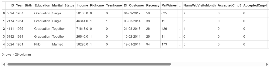
data = pd.read_csv('/home/mw/project/marketing_campaign.csv', sep='\t')data.head()
查看数据基本信息
data.info()<class 'pandas.core.frame.DataFrame'>RangeIndex: 2240 entries, 0 to 2239Data columns (total 29 columns):# Column Non-Null Count Dtype--- ------ -------------- -----0 ID 2240 non-null int641 Year_Birth 2240 non-null int642 Education 2240 non-null object3 Marital_Status 2240 non-null object4 Income 2216 non-null float645 Kidhome 2240 non-null int646 Teenhome 2240 non-null int647 Dt_Customer 2240 non-null object8 Recency 2240 non-null int649 MntWines 2240 non-null int6410 MntFruits 2240 non-null int6411 MntMeatProducts 2240 non-null int6412 MntFishProducts 2240 non-null int6413 MntSweetProducts 2240 non-null int6414 MntGoldProds 2240 non-null int6415 NumDealsPurchases 2240 non-null int6416 NumWebPurchases 2240 non-null int6417 NumCatalogPurchases 2240 non-null int6418 NumStorePurchases 2240 non-null int6419 NumWebVisitsMonth 2240 non-null int6420 AcceptedCmp3 2240 non-null int6421 AcceptedCmp4 2240 non-null int6422 AcceptedCmp5 2240 non-null int6423 AcceptedCmp1 2240 non-null int6424 AcceptedCmp2 2240 non-null int6425 Complain 2240 non-null int6426 Z_CostContact 2240 non-null int6427 Z_Revenue 2240 non-null int6428 Response 2240 non-null int64dtypes: float64(1), int64(25), object(3)memory usage: 507.6+ KB
print(f"数据集行数:{data.shape[0]}")print(f"数据集列数:{data.shape[1]}")
数据集行数:2240数据集列数:29
3、数据处理
删除 ID 、Z_CostContact、Z_Revenue 列
data = data.drop(labels=['ID', 'Z_CostContact', 'Z_Revenue'], axis=1)将Dt_Customer 转换为时间日期类型
data['Dt_Customer'] = pd.to_datetime(data['Dt_Customer'], format='%d-%m-%Y')data['Dt_Customer'].dtype
dtype('<M8[ns]')检查是否存在缺失值
data.isnull().sum()Year_Birth 0Education 0Marital_Status 0Income 24Kidhome 0Teenhome 0Dt_Customer 0Recency 0MntWines 0MntFruits 0MntMeatProducts 0MntFishProducts 0MntSweetProducts 0MntGoldProds 0NumDealsPurchases 0NumWebPurchases 0NumCatalogPurchases 0NumStorePurchases 0NumWebVisitsMonth 0AcceptedCmp3 0AcceptedCmp4 0AcceptedCmp5 0AcceptedCmp1 0AcceptedCmp2 0Complain 0Response 0dtype: int64
# 分析缺失比例print(f"缺失比例:{round(data['Income'].isnull().mean(), 2)*100}%")
缺失比例:1.0%
缺失比例为 1.0% 小于 5% ,直接删除缺失值
删除法处理缺失值
data = data[~data['Income'].isnull()]data.isnull().sum()Year_Birth 0Education 0Marital_Status 0Income 0Kidhome 0Teenhome 0Dt_Customer 0Recency 0MntWines 0MntFruits 0MntMeatProducts 0MntFishProducts 0MntSweetProducts 0MntGoldProds 0NumDealsPurchases 0NumWebPurchases 0NumCatalogPurchases 0NumStorePurchases 0NumWebVisitsMonth 0AcceptedCmp3 0AcceptedCmp4 0AcceptedCmp5 0AcceptedCmp1 0AcceptedCmp2 0Complain 0Response 0dtype: int64
检查是否存在重复值
print(f"数据集重复值的数量:{data.duplicated().sum()}")数据集重复值的数量:182
data[data.duplicated()]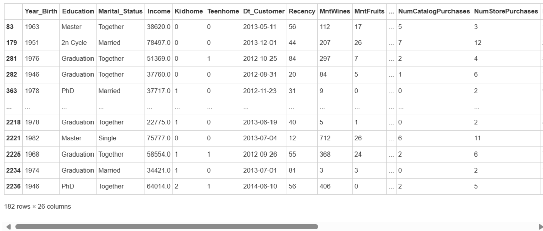
删除重复值,保留最后一次出现的记录
data = data.drop_duplicates(keep='last')data.duplicated().sum()
检查是否存在异常值
# 特征字典feature = {'Year_Birth':'出生年份','Income':'家庭年收入','Recency':'上次购买以来的天数','MntWines':'在葡萄酒上的花费','MntFruits':'在水果上的花费','MntMeatProducts':'在肉类上的支出','MntFishProducts':'在鱼上的花费','MntSweetProducts':'在糖果上的花费','MntGoldProds':'在黄金上花费的金额','NumDealsPurchases':'使用折扣进行的购买次数','NumWebPurchases':'通过公司网站进行的购买次数','NumCatalogPurchases':'使用目录进行的购买次数','NumStorePurchases':'直接在商店中进行的购买次数','NumWebVisitsMonth':'上个月公司网站的访问次数'}plt.figure(figsize=(20, 15))for i, (col, col_name) in enumerate(feature.items(), start=1):plt.subplot(3, 5, i)sns.boxplot(data=data[col])plt.grid(axis='y', linestyle='--', alpha=0.8)plt.title(f"{col_name}箱线图", fontproperties=my_font)plt.tight_layout()plt.show()
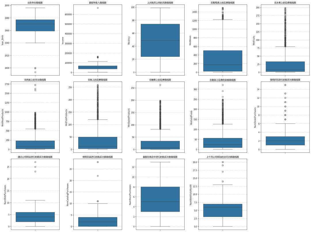
对客户出生年份进行处理
根据数据集的更新时间为 2021 年,以 100 岁为上限,即出生年份早于 1921 年的客户为异常值
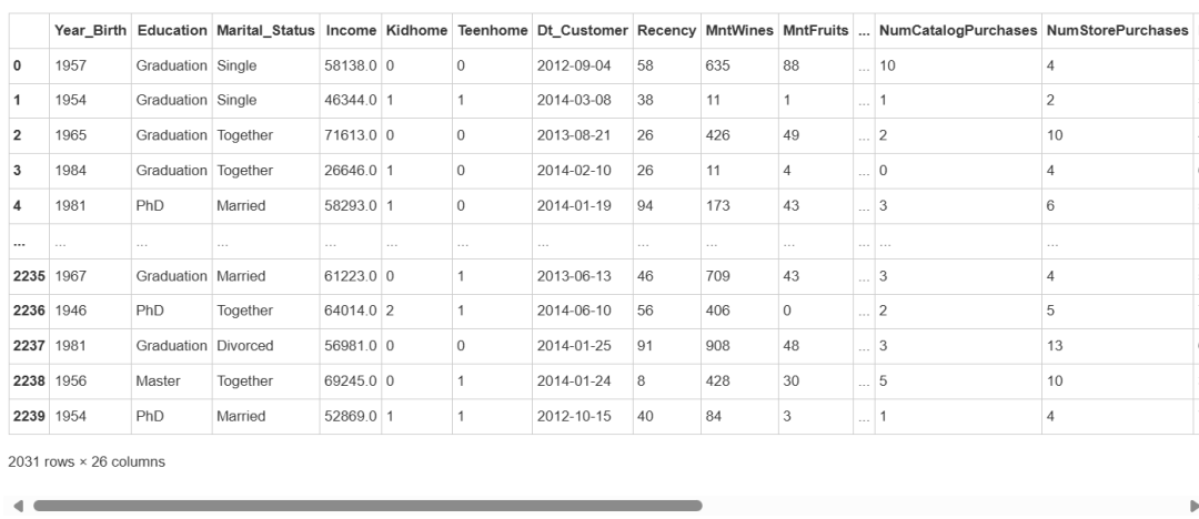
series = pd.to_datetime(data['Year_Birth'], format='%Y').dt.yeardata = data[~(series < 1921)]data
由于客户行为的多样性,其他特征数据异常值可以不做处理
查看类别特征数据情况
labels=['Education', 'Marital_Status', 'Kidhome','Teenhome', 'AcceptedCmp3', 'AcceptedCmp4','AcceptedCmp5', 'AcceptedCmp1', 'AcceptedCmp2','Complain', 'Response']for col in labels:print(f"{col}的唯一值个数:{data[col].nunique()}")print(f"唯一值:{data[col].unique()}")print('-'*45)
Education的唯一值个数:5唯一值:['Graduation' 'PhD' 'Master' 'Basic' '2n Cycle']---------------------------------------------Marital_Status的唯一值个数:8唯一值:['Single' 'Together' 'Married' 'Divorced' 'Widow' 'Alone' 'Absurd' 'YOLO']---------------------------------------------Kidhome的唯一值个数:3唯一值:[0 1 2]---------------------------------------------Teenhome的唯一值个数:3唯一值:[0 1 2]---------------------------------------------AcceptedCmp3的唯一值个数:2唯一值:[0 1]---------------------------------------------AcceptedCmp4的唯一值个数:2唯一值:[0 1]---------------------------------------------AcceptedCmp5的唯一值个数:2唯一值:[0 1]---------------------------------------------AcceptedCmp1的唯一值个数:2唯一值:[0 1]---------------------------------------------AcceptedCmp2的唯一值个数:2唯一值:[0 1]---------------------------------------------Complain的唯一值个数:2唯一值:[0 1]---------------------------------------------Response的唯一值个数:2唯一值:[1 0]---------------------------------------------
4、探索性数据分析(EDA)
描述性分析
data.describe(include=['int', 'float']).T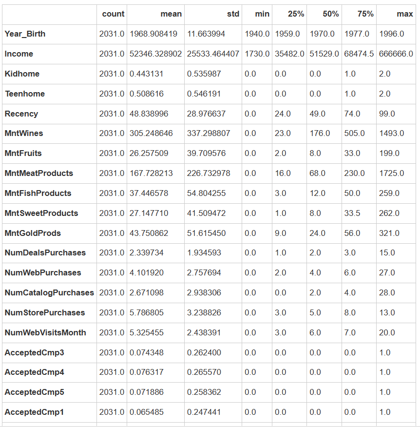
1.客户人口统计学特征
年龄分布
平均出生年份:1968.9年(约52-53岁)
年龄范围:
最年轻客户:1996年出生(约22岁)
最年长客户:1940年出生(约81岁)
中位数年龄:1970年出生(约51岁)
主要客户群:50%客户出生于1959-1977年间(42-62岁)
家庭结构
儿童数量:
平均0.44个/家庭(标准差0.54)
中位数0个,75分位数为1个
青少年数量:
平均0.51个/家庭(标准差0.55)
分布与儿童相似
洞察:约半数家庭有未成年子女(儿童或青少年)
收入状况
平均收入:52,346
收入分布:
中位数:51,529
25%客户收入<35,482
75%客户收入<68,475
贫富差距:标准差25,533显示收入分布不均
2.消费行为分析
产品类别支出(年度)
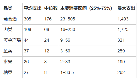
关键发现:
葡萄酒是绝对主导品类,占消费大头
肉类为第二大支出品类
各品类消费呈现明显右偏(均值>中位数)
购买活跃度
最近购买间隔:
平均48.8天(中位数49天)
25%客户≤24天未购买
75%客户≤74天未购买
消费频率:
分布均匀,无明显集中趋势
3.渠道行为分析
购买渠道偏好
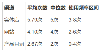
渠道洞察:
实体店仍是主要购买渠道
线上渠道(网站)使用率次之
目录销售有提升空间(25%客户从未使用)
数字互动
月均网站访问:5.33次(中位数6次)
促销使用:
平均使用折扣2.34次(中位数2次)
最高达15次
4.营销活动效果
活动响应率
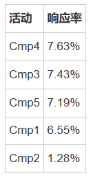
关键发现:
活动4效果最佳,活动2效果显著较差
整体响应率15.36%
投诉率极低(0.94%),表明服务质量良好
data.describe(include='object').T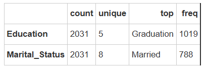
labels = data['Education'].value_counts().index.tolist()counts = data['Education'].value_counts().values.tolist()pie = Pie()pie.add('教育水平', data_pair=[list(x) for x in zip(labels, counts)], label_opts=opts.LabelOpts(formatter="{b}: {d}%", position='inside'))pie.set_global_opts(title_opts=opts.TitleOpts(title='教育水平分布图'))pie.render_notebook()
labels = data['Marital_Status'].value_counts().index.tolist()counts = data['Marital_Status'].value_counts().values.tolist()pie = Pie()pie.add('婚姻状况', data_pair=[list(x) for x in zip(labels, counts)], label_opts=opts.LabelOpts(formatter="{b}: {d}%", position='inside'))pie.set_global_opts(title_opts=opts.TitleOpts(title='婚姻状况分析图', pos_right='center'),legend_opts=opts.LegendOpts(pos_left='5%', pos_top='center', orient='v'))pie.render_notebook()
1.教育水平分析
主要分布:
最高频:本科毕业(Graduation) - 1,019人,占比50.17%
核心客户群为大学毕业生
2.婚姻状况分析
主要分布:
最高频:已婚(Married) - 788人,占比38.8%
已婚客户是最大群体
特征相关性分析
# 相关性矩阵correlation =data.select_dtypes(include='number').corr()plt.figure(figsize=(20, 10))sns.heatmap(data=correlation, cmap='coolwarm', annot=True, fmt='.2f')plt.title('特征相关性热力图')plt.show()
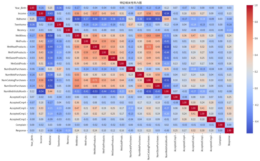
强相关性特征
收入(Income)与其他特征的关系:
收入与多种产品支出高度相关:肉类产品(0.57)、葡萄酒(0.56)、水果(0.42)、鱼类(0.43)、甜食(0.43)
收入与购买渠道相关:目录购买(0.58)、实体店购买(0.52)
收入与家庭中有小孩(Kidhome)呈负相关(-0.43)
产品支出之间的相关性:
不同产品类别支出之间存在中等至强相关性(0.38-0.59),表明购买一种产品的客户往往也会购买其他产品
肉类产品支出与目录购买高度相关(0.73)
购买渠道相关性:
目录购买(NumCatalogPurchases)与多种产品支出高度相关
网络购买(NumWebPurchases)与葡萄酒支出相关(0.55)
弱相关性特征
最近购买时间(Recency):
与几乎所有其他特征的相关性都非常弱,表明这是一个独立变量
营销活动接受度(AcceptedCmp系列):
大多数营销活动的接受度与其他特征相关性较弱
例外是AcceptedCmp5,与多种产品支出和购买渠道有中等相关性(0.17-0.47)
其他特征
家庭结构影响:
家中有小孩(Kidhome)与收入、产品支出呈负相关
家中有青少年(Teenhome)与某些产品(如水果、肉类)支出有弱负相关
年龄(Year_Birth):
与大多数特征相关性较弱
5、聚类分析
特征工程
# 复制数据new_data = data.copy()# 以数据集的更新时间(2021 年)为标准,将出生年份转换为年龄new_data['Age'] = 2021 - new_data['Year_Birth']# 将客户注册日期转换为天数update_date = datetime(2021, 1, 1) # 指定日期为 2021 年 1 月 1 日new_data['Dt_Customer'] = (update_date - new_data['Dt_Customer']).dt.days# 将全部的消费类型特征合并new_data['Consumption_amount'] = new_data['MntWines'] + new_data['MntFruits'] + new_data['MntMeatProducts'] + new_data['MntFishProducts'] + new_data['MntSweetProducts'] + new_data['MntGoldProds']# 将婚姻状态修改为单身、配偶的状态new_data['Living_condition'] = new_data['Marital_Status'].replace({'Married':'Partner', 'Together':'Partner', 'Absurd':'Single', 'Widow':'Single', 'YOLO':'Single', 'Divorced':'Single', 'Alone':'Single'})# 将教育水平分为本科生、研究生、毕业生new_data['Education'] = new_data['Education'].replace({'Basic':'Undergraduate','2n Cycle':'Undergraduate', 'Graduation':'Graduate', 'Master':'Postgraduate', 'PhD':'Postgraduate'})# 将Kidhome、Teenhome特征合并new_data['family_child'] = new_data['Kidhome'] +new_data['Teenhome']# 添加特征Is_Parent,用于判断客户是否为家长new_data['Is_Parent'] = (new_data['family_child'] > 0).astype(int)to_drop = ['Year_Birth', 'Marital_Status', 'Kidhome', 'Teenhome', 'MntWines', 'MntFruits', 'MntMeatProducts', 'MntFishProducts', 'MntSweetProducts', 'MntGoldProds']new_data = new_data.drop(to_drop, axis=1)
数据准备:选择用于聚类的特征
labels=['AcceptedCmp3', 'AcceptedCmp4', 'AcceptedCmp5', 'AcceptedCmp1', 'AcceptedCmp2', 'Response']X = new_data.drop(labels=labels, axis=1)
数据预处理:对数值型特征标准化,对类别型特征标签编码
# 标签编码encoder = LabelEncoder()for col in ['Education', 'Living_condition']:X[col] = encoder.fit_transform(X[col])# 编码顺序result = dict(zip(encoder.classes_, range(len(encoder.classes_))))print(f"{col}特征编码结果:{result}")# 标准化scaler = StandardScaler()X_scaled = scaler.fit_transform(X)
Education特征编码结果:{'Graduate': 0, 'Postgraduate': 1, 'Undergraduate': 2}Living_condition特征编码结果:{'Partner': 0, 'Single': 1}
选择聚类数K:通过肘部法则和轮廓系数判断最佳的K值
# 计算不同K值的惯性(簇内平方和)和轮廓系数inertias = list()silhouette_scores = list()k_range = range(2, 11)for k in k_range:kmeans = KMeans(n_clusters=k, random_state=42)kmeans.fit(X_scaled)inertias.append(kmeans.inertia_)silhouette_scores.append(silhouette_score(X_scaled, kmeans.labels_))# 格式化数据inertias = [round(x) for x in inertias]silhouette_scores = [round(x, 4) for x in silhouette_scores]# 绘制肘部曲线line = (Line().add_xaxis(k_range).add_yaxis('惯性(簇内平方和)', inertias, is_smooth=True).extend_axis(yaxis=opts.AxisOpts(position='right')).add_yaxis('轮廓系数', silhouette_scores, is_smooth=True, yaxis_index=1).set_global_opts(title_opts=opts.TitleOpts(title='最佳K值选择图'),xaxis_opts=opts.AxisOpts(name='聚类中心数', name_location='center'),tooltip_opts=opts.TooltipOpts(trigger='axis')))line.render_notebook()
惯性值快速下降,体现“肘部效应”:
K=3 后下降速度逐渐趋缓,出现“肘部”现象,意味着继续增加 K 值带来的改善边际效益不大。
轮廓系数最大原则:
K=3 时轮廓系数为 0.1942,具有很好的聚类效果。
根据上述分析,K=3 是当前聚类效果最优的选择:其轮廓系数为 0.1942,说明聚类结果在类内紧凑、类间分离方面优秀;同时惯性值为 20907,类内误差较小,表现良好。
最佳 KMeans 模型
kmeans = KMeans(n_clusters=3, random_state=42)kmeans.fit(X_scaled)# 获取聚类结果cluster_labels = kmeans.labels_cluster_centroids = kmeans.cluster_centers_# 返回聚类结果用做特征重要性分析X['Cluster'] = cluster_labels
可视化聚类效果
# PCA降维pca = PCA(n_components=3)X_pca = pca.fit_transform(X_scaled)cluster_centroids_pca = pca.transform(cluster_centroids)print(f"累计解释率(信息保留总量):{round(sum(pca.explained_variance_ratio_), 2)}")
累计解释率(信息保留总量):0.5
信息保留总量为 0.5,可以用于可视化聚类效果
# 构造3D散点图的数据格式data_3d = [list(X_pca[i])+[int(cluster_labels[i])] for i in range(len(X_scaled))]# 绘图3D散点图colors = ['#FF6F61', '#6B5B95', '#88B04B'] # 定义颜色scatter3d = (Scatter3D().add(series_name="聚类结果",data=data_3d,xaxis3d_opts=opts.Axis3DOpts(name="主成分1"),yaxis3d_opts=opts.Axis3DOpts(name="主成分2"),zaxis3d_opts=opts.Axis3DOpts(name="主成分3"),grid3d_opts=opts.Grid3DOpts(width=100, depth=100, height=100),itemstyle_opts=opts.ItemStyleOpts(opacity=0.8)).add(series_name='聚类中心点',data=cluster_centroids_pca.tolist(),itemstyle_opts=opts.ItemStyleOpts(color='black', opacity=1)).set_global_opts(title_opts=opts.TitleOpts(title="K-means聚类效果(PCA降维3D可视化)"),visualmap_opts=opts.VisualMapOpts(dimension=3,max_=int(max(cluster_labels)),min_=int(min(cluster_labels)),range_color=colors,series_index=0)))scatter3d.render_notebook()
6、用户画像
特征重要性
X_train, X_test, y_train, y_test = train_test_split(X_scaled, cluster_labels, test_size=0.3, random_state=42)clf = RandomForestClassifier()clf.fit(X_train, y_train)result = permutation_importance(estimator=clf, X=X_test, y=y_test, n_repeats=10, random_state=42)feature_importances = pd.DataFrame(data={'特征':X.drop(labels='Cluster', axis=1).columns, '重要性':result['importances_mean']}).sort_values(by='重要性', ascending=False)plt.figure(figsize=(10, 6))sns.barplot(data=feature_importances, x='重要性', y='特征', orient='h', hue='特征')plt.title('特征重要性')plt.show()
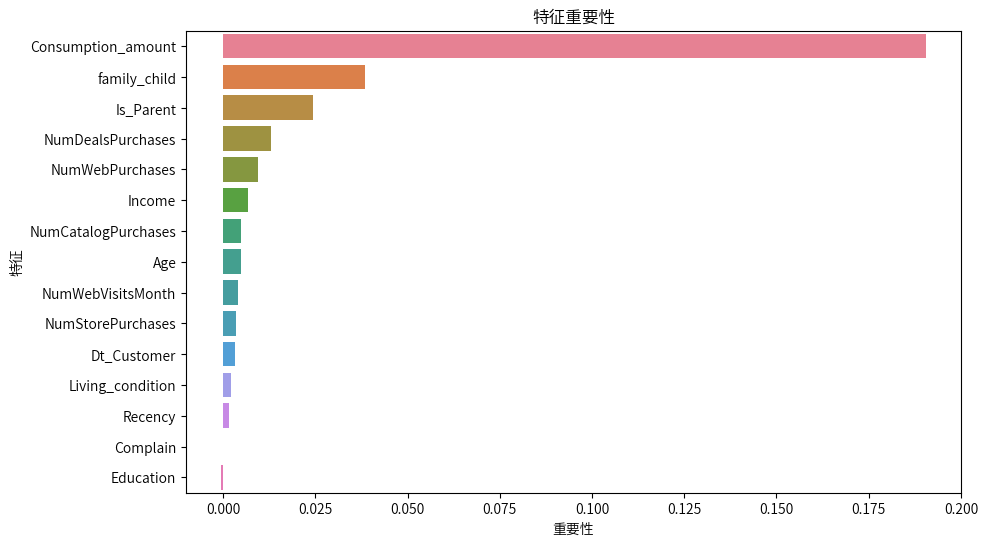
关键行为特征分析:
Consumption_amount(消费金额)
重要性最高,远高于其他特征,说明客户的消费水平在分群中起到主导作用。
代表高消费和低消费客户群体之间的显著区分。
family_child(家庭中是否有孩子)
对客户分群也有较大影响,表明家庭结构可能影响消费习惯。
Is_Parent(是否为父母)
与 family_child 相关联,也说明家庭角色在客户分群中是一个重要维度。
NumDealsPurchases(折扣购买次数)
该特征重要性较高,表示价格敏感度和促销响应是客户分类的重要依据。
Income(收入)
收入水平影响消费能力,与 Consumption_amount 密切相关,虽然重要性略低,但依旧显著。
NumWebVisitsMonth / NumWebPurchases
网络访问和购物行为代表客户的线上活跃度,适用于区分传统购物者与线上活跃用户。
NumCatalogPurchases(目录购买次数)
显示用户对特定购物方式(如目录购物)的偏好,可能反映年龄或生活方式的差异。
次要或影响较小的特征(权重接近 0):
Living condition, Education, Age, Dt_Customer, Complain(投诉), NumStorePurchases(实体店购买), Recency(最近一次消费):
这些特征对分群影响相对较小。
总结:
影响客户分群的关键行为特征包括:
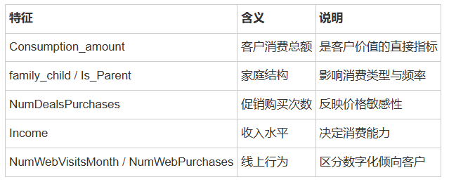
可视化分析
# 将聚类结果添加到数据中new_data['Cluster'] = cluster_labels
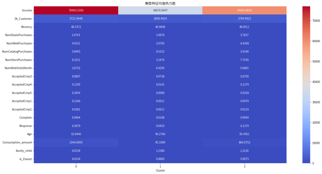
聚类特征均值
#选择数值类型特征cluster_means = new_data.select_dtypes(include=['int', 'float']).groupby(by='Cluster').agg('mean')plt.figure(figsize=(20, 10))sns.heatmap(data=cluster_means.T, cmap='coolwarm', annot=True, fmt='.4f')plt.title('聚类特征均值热力图')plt.show()
不同簇之间各特征的分布
# 获取所有教育水平类别edu_levels = new_data['Education'].unique().tolist()# 按照每个教育水平统计在不同簇中的数量y_data0 = [new_data[(new_data['Cluster'] == 0) & (new_data['Education'] == edu)].shape[0] for edu in edu_levels]y_data1 = [new_data[(new_data['Cluster'] == 1) & (new_data['Education'] == edu)].shape[0] for edu in edu_levels]y_data2 = [new_data[(new_data['Cluster'] == 2) & (new_data['Education'] == edu)].shape[0] for edu in edu_levels]# 绘图bar = (Bar().add_xaxis(edu_levels).add_yaxis("Cluster 0", y_data0).add_yaxis("Cluster 1", y_data1).add_yaxis("Cluster 2", y_data2).set_global_opts(title_opts=opts.TitleOpts(title="不同簇的教育水平分布"),xaxis_opts=opts.AxisOpts(name="教育水平"),yaxis_opts=opts.AxisOpts(name="人数"),toolbox_opts=opts.ToolboxOpts()))bar.render_notebook()
# 获取所有生活状态类别conditions = new_data['Living_condition'].unique().tolist()# 按照每个生活状态统计在不同簇中的数量y_data0 = [new_data[(new_data['Cluster'] == 0) & (new_data['Living_condition'] == con)].shape[0] for con in conditions]y_data1 = [new_data[(new_data['Cluster'] == 1) & (new_data['Living_condition'] == con)].shape[0] for con in conditions]y_data2 = [new_data[(new_data['Cluster'] == 2) & (new_data['Living_condition'] == con)].shape[0] for con in conditions]# 绘图bar = (Bar().add_xaxis(conditions).add_yaxis("Cluster 0", y_data0).add_yaxis("Cluster 1", y_data1).add_yaxis("Cluster 2", y_data2).set_global_opts(title_opts=opts.TitleOpts(title='不同簇的生活状态分布'),xaxis_opts=opts.AxisOpts(name='生活状态'),yaxis_opts=opts.AxisOpts(name='人数'),toolbox_opts=opts.ToolboxOpts()))bar.render_notebook()
# 获取所有簇类别clusters = new_data['Cluster'].unique().tolist()labels = ['Cluster '+str(x) for x in clusters]# 按照每个簇统计在不同簇中使用折扣购买次数deal_counts = list()for cluster in clusters:counts = new_data[(new_data['Cluster'] == cluster)]['NumDealsPurchases'].sum()deal_counts.append(int(counts))pie = Pie()pie.add('', data_pair=[list(x) for x in zip(labels, deal_counts)], label_opts=opts.LabelOpts(formatter="{b}: {d}%", position='inside'))pie.set_global_opts(title_opts=opts.TitleOpts(title='不同簇中使用折扣购买次数分布', pos_right='center'),legend_opts=opts.LegendOpts(pos_left='5%', pos_top='center', orient='v'))pie.render_notebook()
# 获取所有簇类别clusters = new_data['Cluster'].unique().tolist()labels = ['Cluster '+str(x) for x in clusters]# 按照每个簇统计在不同簇中使用网站购买次数web_counts = list()for cluster in clusters:counts = new_data[(new_data['Cluster'] == cluster)]['NumWebPurchases'].sum()web_counts.append(int(counts))pie = Pie()pie.add('', data_pair=[list(x) for x in zip(labels, web_counts)], label_opts=opts.LabelOpts(formatter="{b}: {d}%", position='inside'))pie.set_global_opts(title_opts=opts.TitleOpts(title='不同簇中使用网站购买次数分布', pos_right='center'),legend_opts=opts.LegendOpts(pos_left='5%', pos_top='center', orient='v'))pie.render_notebook()
# 获取所有簇类别clusters = new_data['Cluster'].unique().tolist()labels = ['Cluster '+str(x) for x in clusters]# 按照每个簇统计在不同簇中使用目录购买次数catalog_counts = list()for cluster in clusters:counts = new_data[(new_data['Cluster'] == cluster)]['NumCatalogPurchases'].sum()catalog_counts.append(int(counts))pie = Pie()pie.add('', data_pair=[list(x) for x in zip(labels, catalog_counts)], label_opts=opts.LabelOpts(formatter="{b}: {d}%", position='inside'))pie.set_global_opts(title_opts=opts.TitleOpts(title='不同簇中使用目录购买次数分布', pos_right='center'),legend_opts=opts.LegendOpts(pos_left='5%', pos_top='center', orient='v'))pie.render_notebook()
# 获取所有簇类别clusters = new_data['Cluster'].unique().tolist()labels = ['Cluster '+str(x) for x in clusters]# 按照每个簇统计在不同簇中在实体店购买次数store_counts = list()for cluster in clusters:counts = new_data[(new_data['Cluster'] == cluster)]['NumStorePurchases'].sum()store_counts.append(int(counts))pie = Pie()pie.add('', data_pair=[list(x) for x in zip(labels, store_counts)], label_opts=opts.LabelOpts(formatter="{b}: {d}%", position='inside'))pie.set_global_opts(title_opts=opts.TitleOpts(title='不同簇中在实体店购买次数分布', pos_right='center'),legend_opts=opts.LegendOpts(pos_left='5%', pos_top='center', orient='v'))pie.render_notebook()
# 获取所有簇类别clusters = new_data['Cluster'].unique().tolist()labels = ['Cluster '+str(x) for x in clusters]# 按照每个簇统计在不同簇中访问网站的次数webvisit_counts = list()for cluster in clusters:counts = new_data[(new_data['Cluster'] == cluster)]['NumWebVisitsMonth'].sum()webvisit_counts.append(int(counts))pie = Pie()pie.add('', data_pair=[list(x) for x in zip(labels, webvisit_counts)], label_opts=opts.LabelOpts(formatter="{b}: {d}%", position='inside'))pie.set_global_opts(title_opts=opts.TitleOpts(title='不同簇中访问网站的次数分布', pos_right='center'),legend_opts=opts.LegendOpts(pos_left='5%', pos_top='center', orient='v'))pie.render_notebook()
画像分析
Cluster 0 - 高价值独立中年客户
特征
消费金额: 极高(1345)
收入: 极高(76994)
年龄: 中老年(53 岁)
教育: 大部分为研究生、毕业生
生活状态: 大部分为 Partner
家庭结构: 基本无子女(family_child ≈ 0),非父母
购买行为: 偏好实体店购买、按照目录价格购买,线上一般
投诉: 极低(≈0)
用户画像:
高消费、高收入、独立中年、偏好线下、无家庭负担
Cluster 1 - 年轻低消费潜力客户
特征
消费金额: 极低(≈95)
收入: 低(34670)
年龄: 相对整体最年轻(≈49 岁)
教育: 大部分为研究生、毕业生
生活状态: 大部分为 Partner
家庭结构: 有子女(family_child ≈ 1.24),是父母
购买行为: 偏好线上访问但不活跃购买(Web访问最高,购买少)
投诉: 相对整体较多(≈0.01)
用户画像:
年轻家庭、教育水平高、消费低、线上活跃但购买少
Cluster 2 - 中产家庭购买偏好全面型客户
特征
消费金额: 中等(804)
收入: 中等(59694)
年龄: 中老年(≈55 岁)
教育: 大部分为研究生、毕业生
生活状态: 大部分为 Partner
家庭结构: 有子女(family_child ≈ 1.22),是父母
购买行为: 全面型购买偏好、数字化转型
投诉: 相对整体中等偏低
用户画像:
中等消费、中年家庭客户、全面型购买偏好、数字化转型
案例来源:
https://www.heywhale.com/mw/project/6828621ed303614c52f36691

魔乐社区(Modelers.cn) 是一个中立、公益的人工智能社区,提供人工智能工具、模型、数据的托管、展示与应用协同服务,为人工智能开发及爱好者搭建开放的学习交流平台。社区通过理事会方式运作,由全产业链共同建设、共同运营、共同享有,推动国产AI生态繁荣发展。
更多推荐


 20
20 0
0- 0


 已为社区贡献3条内容

所有评论(0)