背景

YOLO，You Only look once。顾名思义，你只需要看一次，即one stage推理模型。它是在two stage基础上提出，相比two stage少了寻找目标的阶段，所以推理极大地加快了推理速度。yolo算法以快准出名，能够实现实时推理，适用于多种场景。yolo从推出后就备受青睐，发展也十分迅速，从推出后几年就从yolov1发展到了yolov10，接下来讨论一下这些算法有什么特点以及创新。

YOLOv1

yolov1发布于2015年，相关论文《You Only Look Once: Unified, Real-Time Object Detection》（https://arxiv.org/abs/1506.02640）。本文主要分析算法的模型结构和思想。

模型结构

yolov1是采用了grid的方法，将图像划分为$S\times S$个grid，每个grid对应俩个框，每个框有五个参数，分别是长$h$、宽$w$、中心点横坐标$x$、中心点纵坐标$y$，框对应的置信度$C$。所以一个grid对应的输出为$num(class)+10$。即一个grid对应的俩个框共享一个分类概率。这里需要对置信度进行定义，置信度是代表当前框包含目标的概率，所以$C$可以定义为$IO{U}_{true}^{pred}$，即$$C=Pr(Object)\ast IO{U}_{true}^{pred}$$当目标grid中包含真实值的中心点时，$Pr(Object)=1$，否则$Pr(Object)=0$。

了解了上述的这些之后，再看下面这张图，就可以比较清晰的理解它的思想了。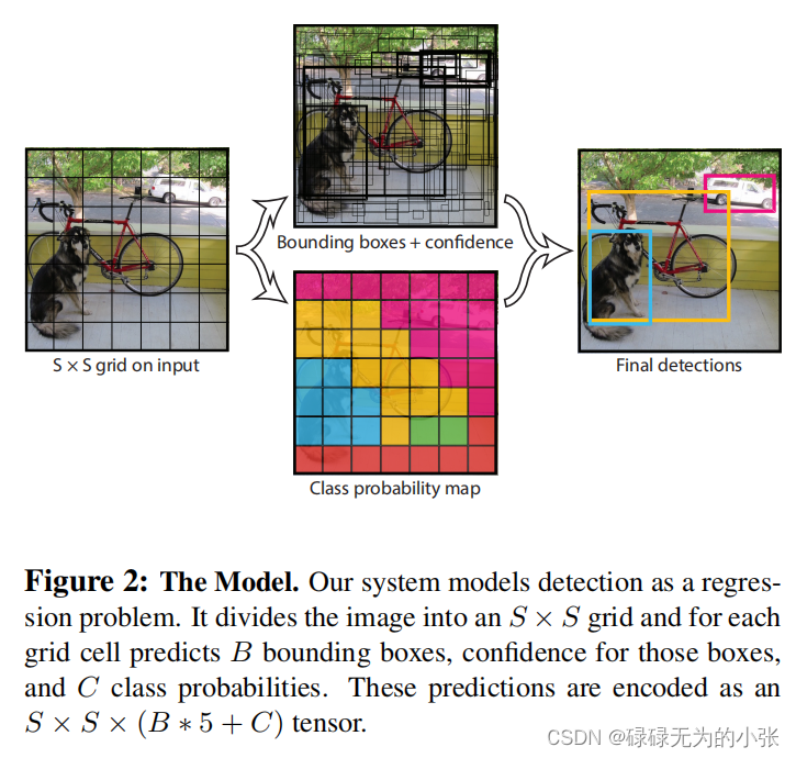

下图是模型的具体结构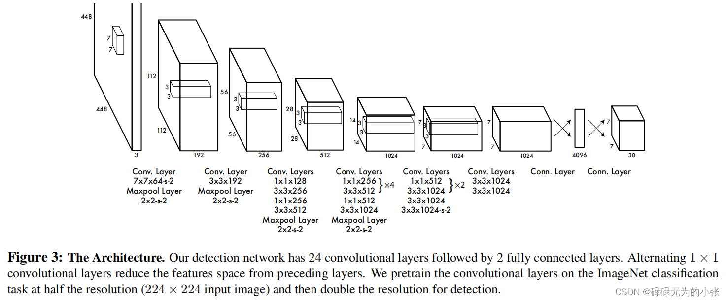

这里的图上的维度变换可以参考（https://blog.csdn.net/Jiangnan_Cai/article/details/136763127）给出的表，再结合上图的表就可以比较好的理解了。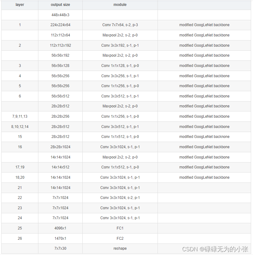

最终得到$（7\times 7\times 30）$的输出，这里把可以理解一个grid对应一个object，俩个框是为了选出更好的一个。

Loss Function

先看论文中给出的loss function defineKaTeX parse error: No such environment: align* at position 7: \begin{̲a̲l̲i̲g̲n̲*̲}̲Loss =& \lambda…
其中$$1_i^{obj}=\{\begin{array}{cc}1& if\text{ 第}i个grid包含目标\\ 0& else\end{array}$$$$1_{ij}^{obj}=\{\begin{array}{cc}1& if\text{ 第}i个grid包含目标且第j个框为B个框中IOU最大的框\\ 0& else\end{array}$$
理解了这俩个$1$的含义，结合下面的loss function的代码就可以较好的了解了。

import torch
import torch.nn as nn
import torch.nn.functional as F
from torch.autograd import Variable


class Loss(nn.Module):

    def __init__(self, feature_size=7, num_bboxes=2, num_classes=20, lambda_coord=5.0, lambda_noobj=0.5):
        """ Constructor.
        Args:
            feature_size: (int) size of input feature map.
            num_bboxes: (int) number of bboxes per each cell.
            num_classes: (int) number of the object classes.
            lambda_coord: (float) weight for bbox location/size losses.
            lambda_noobj: (float) weight for no-objectness loss.
        """
        super(Loss, self).__init__()

        self.S = feature_size
        self.B = num_bboxes
        self.C = num_classes
        self.lambda_coord = lambda_coord
        self.lambda_noobj = lambda_noobj


    def compute_iou(self, bbox1, bbox2):
        """ Compute the IoU (Intersection over Union) of two set of bboxes, each bbox format: [x1, y1, x2, y2].
        Args:
            bbox1: (Tensor) bounding bboxes, sized [N, 4].
            bbox2: (Tensor) bounding bboxes, sized [M, 4].
        Returns:
            (Tensor) IoU, sized [N, M].
        """
        N = bbox1.size(0)
        M = bbox2.size(0)

        # Compute left-top coordinate of the intersections
        lt = torch.max(
            bbox1[:, :2].unsqueeze(1).expand(N, M, 2), # [N, 2] -> [N, 1, 2] -> [N, M, 2]
            bbox2[:, :2].unsqueeze(0).expand(N, M, 2)  # [M, 2] -> [1, M, 2] -> [N, M, 2]
        )
        # Conpute right-bottom coordinate of the intersections
        rb = torch.min(
            bbox1[:, 2:].unsqueeze(1).expand(N, M, 2), # [N, 2] -> [N, 1, 2] -> [N, M, 2]
            bbox2[:, 2:].unsqueeze(0).expand(N, M, 2)  # [M, 2] -> [1, M, 2] -> [N, M, 2]
        )
        # Compute area of the intersections from the coordinates
        wh = rb - lt   # width and height of the intersection, [N, M, 2]
        wh[wh < 0] = 0 # clip at 0
        inter = wh[:, :, 0] * wh[:, :, 1] # [N, M]

        # Compute area of the bboxes
        area1 = (bbox1[:, 2] - bbox1[:, 0]) * (bbox1[:, 3] - bbox1[:, 1]) # [N, ]
        area2 = (bbox2[:, 2] - bbox2[:, 0]) * (bbox2[:, 3] - bbox2[:, 1]) # [M, ]
        area1 = area1.unsqueeze(1).expand_as(inter) # [N, ] -> [N, 1] -> [N, M]
        area2 = area2.unsqueeze(0).expand_as(inter) # [M, ] -> [1, M] -> [N, M]

        # Compute IoU from the areas
        union = area1 + area2 - inter # [N, M, 2]
        iou = inter / union           # [N, M, 2]

        return iou

    def forward(self, pred_tensor, target_tensor):
        """ Compute loss for YOLO training.
        Args:
            pred_tensor: (Tensor) predictions, sized [n_batch, S, S, Bx5+C], 5=len([x, y, w, h, conf]).
            target_tensor: (Tensor) targets, sized [n_batch, S, S, Bx5+C].
        Returns:
            (Tensor): loss, sized [1, ].
        """
        # TODO: Romove redundant dimensions for some Tensors.

        S, B, C = self.S, self.B, self.C
        N = 5 * B + C    # 5=len([x, y, w, h, conf]

        batch_size = pred_tensor.size(0)
        coord_mask = target_tensor[:, :, :, 4] > 0  # mask for the cells which contain objects. [n_batch, S, S]
        noobj_mask = target_tensor[:, :, :, 4] == 0 # mask for the cells which do not contain objects. [n_batch, S, S]
        coord_mask = coord_mask.unsqueeze(-1).expand_as(target_tensor) # [n_batch, S, S] -> [n_batch, S, S, N]
        noobj_mask = noobj_mask.unsqueeze(-1).expand_as(target_tensor) # [n_batch, S, S] -> [n_batch, S, S, N]

        coord_pred = pred_tensor[coord_mask].view(-1, N)            # pred tensor on the cells which contain objects. [n_coord, N]
                                                                    # n_coord: number of the cells which contain objects.
        bbox_pred = coord_pred[:, :5*B].contiguous().view(-1, 5)    # [n_coord x B, 5=len([x, y, w, h, conf])]
        class_pred = coord_pred[:, 5*B:]                            # [n_coord, C]

        coord_target = target_tensor[coord_mask].view(-1, N)        # target tensor on the cells which contain objects. [n_coord, N]
                                                                    # n_coord: number of the cells which contain objects.
        bbox_target = coord_target[:, :5*B].contiguous().view(-1, 5)# [n_coord x B, 5=len([x, y, w, h, conf])]
        class_target = coord_target[:, 5*B:]                        # [n_coord, C]

        # Compute loss for the cells with no object bbox.
        noobj_pred = pred_tensor[noobj_mask].view(-1, N)        # pred tensor on the cells which do not contain objects. [n_noobj, N]
                                                                # n_noobj: number of the cells which do not contain objects.
        noobj_target = target_tensor[noobj_mask].view(-1, N)    # target tensor on the cells which do not contain objects. [n_noobj, N]
                                                                # n_noobj: number of the cells which do not contain objects.
        noobj_conf_mask = torch.cuda.ByteTensor(noobj_pred.size()).fill_(0) # [n_noobj, N]
        for b in range(B):
            noobj_conf_mask[:, 4 + b*5] = 1 # noobj_conf_mask[:, 4] = 1; noobj_conf_mask[:, 9] = 1
        noobj_pred_conf = noobj_pred[noobj_conf_mask]       # [n_noobj, 2=len([conf1, conf2])]
        noobj_target_conf = noobj_target[noobj_conf_mask]   # [n_noobj, 2=len([conf1, conf2])]
        loss_noobj = F.mse_loss(noobj_pred_conf, noobj_target_conf, reduction='sum')

        # Compute loss for the cells with objects.
        coord_response_mask = torch.cuda.ByteTensor(bbox_target.size()).fill_(0)    # [n_coord x B, 5]
        coord_not_response_mask = torch.cuda.ByteTensor(bbox_target.size()).fill_(1)# [n_coord x B, 5]
        bbox_target_iou = torch.zeros(bbox_target.size()).cuda()                    # [n_coord x B, 5], only the last 1=(conf,) is used

        # Choose the predicted bbox having the highest IoU for each target bbox.
        for i in range(0, bbox_target.size(0), B):
            pred = bbox_pred[i:i+B] # predicted bboxes at i-th cell, [B, 5=len([x, y, w, h, conf])]
            pred_xyxy = Variable(torch.FloatTensor(pred.size())) # [B, 5=len([x1, y1, x2, y2, conf])]
            # Because (center_x,center_y)=pred[:, 2] and (w,h)=pred[:,2:4] are normalized for cell-size and image-size respectively,
            # rescale (center_x,center_y) for the image-size to compute IoU correctly.
            pred_xyxy[:,  :2] = pred[:, :2]/float(S) - 0.5 * pred[:, 2:4]
            pred_xyxy[:, 2:4] = pred[:, :2]/float(S) + 0.5 * pred[:, 2:4]

            target = bbox_target[i] # target bbox at i-th cell. Because target boxes contained by each cell are identical in current implementation, enough to extract the first one.
            target = bbox_target[i].view(-1, 5) # target bbox at i-th cell, [1, 5=len([x, y, w, h, conf])]
            target_xyxy = Variable(torch.FloatTensor(target.size())) # [1, 5=len([x1, y1, x2, y2, conf])]
            # Because (center_x,center_y)=target[:, 2] and (w,h)=target[:,2:4] are normalized for cell-size and image-size respectively,
            # rescale (center_x,center_y) for the image-size to compute IoU correctly.
            target_xyxy[:,  :2] = target[:, :2]/float(S) - 0.5 * target[:, 2:4]
            target_xyxy[:, 2:4] = target[:, :2]/float(S) + 0.5 * target[:, 2:4]

            iou = self.compute_iou(pred_xyxy[:, :4], target_xyxy[:, :4]) # [B, 1]
            max_iou, max_index = iou.max(0)
            max_index = max_index.data.cuda()

            coord_response_mask[i+max_index] = 1
            coord_not_response_mask[i+max_index] = 0

            # "we want the confidence score to equal the intersection over union (IOU) between the predicted box and the ground truth"
            # from the original paper of YOLO.
            bbox_target_iou[i+max_index, torch.LongTensor([4]).cuda()] = (max_iou).data.cuda()
        bbox_target_iou = Variable(bbox_target_iou).cuda()

        # BBox location/size and objectness loss for the response bboxes.
        bbox_pred_response = bbox_pred[coord_response_mask].view(-1, 5)      # [n_response, 5]
        bbox_target_response = bbox_target[coord_response_mask].view(-1, 5)  # [n_response, 5], only the first 4=(x, y, w, h) are used
        target_iou = bbox_target_iou[coord_response_mask].view(-1, 5)        # [n_response, 5], only the last 1=(conf,) is used
        loss_xy = F.mse_loss(bbox_pred_response[:, :2], bbox_target_response[:, :2], reduction='sum')
        loss_wh = F.mse_loss(torch.sqrt(bbox_pred_response[:, 2:4]), torch.sqrt(bbox_target_response[:, 2:4]), reduction='sum')
        loss_obj = F.mse_loss(bbox_pred_response[:, 4], target_iou[:, 4], reduction='sum')

        # Class probability loss for the cells which contain objects.
        loss_class = F.mse_loss(class_pred, class_target, reduction='sum')

        # Total loss
        loss = self.lambda_coord * (loss_xy + loss_wh) + loss_obj + self.lambda_noobj * loss_noobj + loss_class
        loss = loss / float(batch_size)

        return loss

yolov1只能预测$S^2$个目标，当一个grid出现多个目标时是无法处理的。

YOLOv2

yolov2是在yolov1上的一些改进，具体看下面的图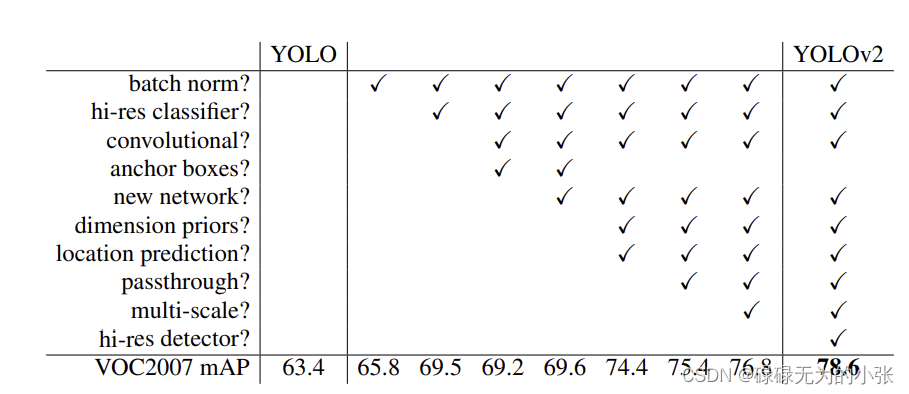

可以看出yolov2主要实验了上述的几个trick，并通过消融实验验证了它们的有效性。BN层

batch norm 和hi-res classifer

batch norm是指对每个batch的数据做norm，由于每个batch的数据可能存在较大的差异，通过batch norm可以降低数据间的方差，从而加快模型的收敛。
hi-res classifer是通过增大输入的分辨率，从而是特征提取模型学习到更多的特征，从而提高模型的准确率。

Convolution with Anchor boxes

yolov2消除了yolov1中的全连接层，同时引入了anchor boxes的方式。这里是消除了yolov1中的所有全连接层，同时移除一个池化层来提高模型输出的分辨率。其使用了$416\times 416$的大小进行模型输入，而非$448\times 448$，这里作者是认为大物体会占据特征图的中心点，使用416的大小经过32倍下采样后是$13\times 13$这样$(6,6)$就是它的中心点。如果是$448\times 448$，那么32倍下采样后是$14\times 14$，这里他的中心点就是四个了。
anchor boxes的思想是来自于faster rcnn，即通过anchor-based的方式，先给定anchor，然后再预测距离中心点的偏移以及相对于给定长宽的比例。

Dimension Clusters

面对不同任务，使用同样的先验框会使模型的预测收敛速度不同，当先验框接近于任务中的目标的大小时，那么收敛会比较快，否则则较慢。但是每个任务都通过手动设定的话，会极大的浪费人力，且不够准确。这里作者提出了通过k-means的方式来寻找先验框。k-means中，最重要的方式就是k的取值以及distance的定义。作者通过实验，认为k值为5时能够达到较好的recall和较低的模型复杂度。同时先验框之间的距离可以通过IOU来判断，即俩个框大小越接近，那么它们的IOU会越大。所以distance定义为$$d(box,centroid)=1-IOU(box,centroid)$$

Direct location prediction

Faster RCNN中预测$x,y$的方式为KaTeX parse error: No such environment: align* at position 7: \begin{̲a̲l̲i̲g̲n̲*̲}̲x =& (t_x*w_a)-…这里如果$t_x$取$1$或$-1$时将会偏移$w_a$的长度，那么$x$的取值就会超出图像了，同理$y$也是。所以这是不可取的，这种方式将会使模型十分不稳定。所以作者提出了新的中心点预测方式，首先先确定中心点所在的框$(c_x,c_y)$表示框在坐标，然后预测$t_x$和$t_y$，通过sigmoid函数将其限制在$(0,1)$上，则有KaTeX parse error: No such environment: align* at position 7: \begin{̲a̲l̲i̲g̲n̲*̲}̲b_x =& \sigma(t…这样就可以预测其中心点的坐标了，注意这里$b_x$和$b_y$是特征图上的坐标，实际坐标还需要进行变换。这里宽和高的长度预测如下KaTeX parse error: No such environment: align* at position 7: \begin{̲a̲l̲i̲g̲n̲*̲}̲b_w =& p_w e^{t…这里$(p_w,p_h)$是先验框的大小，$(b_w,b_h)$则是相对于特征图的大小。timw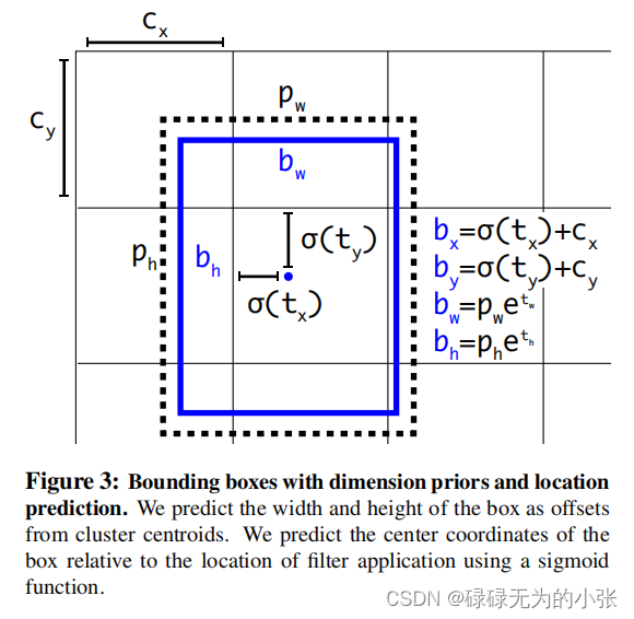
在实际应用中，$b_x,b_y,b_w,b_h$应该看成其相较于当前图的比例，这样在训练时，它的值可以限制在$[0,1]$上，同时在后处理中也可以更加方便，所以有KaTeX parse error: No such environment: align* at position 7: \begin{̲a̲l̲i̲g̲n̲*̲}̲b_x =& \frac{\s…这里$(W,H)$就是指特征图的大小，这里模型的预测还有一个置信度，置信度的定义跟yolov1一样，即$$Pr(obj)\ast IOU(b,obj)=\sigma (t_0)$$

Fine-Grained Features

作者认为$13\times 13$的特征图能较好地学习大目标地特征，但对小目标的学习是不够的，所以提出了passthrough的方式，类似于resnet中的残差连接，将$26\times 26$的特征图合并成$13\times 13$，然后再与最后的输出concat。这里的具体变换是，将特征图$26\times 26\times 512$合并为$13\times 13\times 2048$，具体过程如下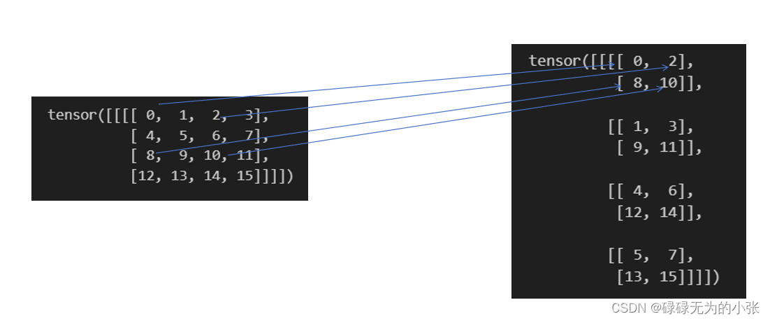

通过这个方式，得到特征图为$13\times 13\times 2048$，再与原来的特征图$13\times 13\times 1024$合并，得到$13\times 13\times 3072$的输出。

Multi-Scale Training

由于yolov2采用了全卷积的方式，所以可以训练任意大小的输入，这可以使模型学习到不同尺度输入的特征，也可以使模型在不同大小输入时具有较强的适应能力。具体方式就是在训练过程中，每10个batch就选取一个尺度，将输入图片resize至这个尺度就可以实现多尺度的训练。由于图像是经过32倍的下采样，所以输入尺度应该是32的倍数，所以这里的尺度选取范围限制在$(320,352,384,\cdots ,608)$中。这个训练trick在许多使用全卷积网络的任务中都可以使用。

Darknet-19

yolov2中提出了新的backbone Darknet-19，其主要采用了$1\times 1$的卷积降低模型的参数量，并使用BN层加快模型的收敛，模型的具体结构如下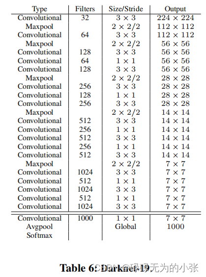

YOLOv3

YOLOv3相较于YOLOv2的变动不大，它延续了Yolov2的location prediction。在Backbone、分类预测和先验框方面做了一些改进。观察（来自https://blog.csdn.net/leviopku/article/details/82660381）Yolov3模型结构图，可以发现Backbone变成了Darknet-53，同时模型的输出头有三个。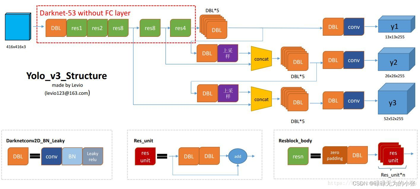

Darknet-53

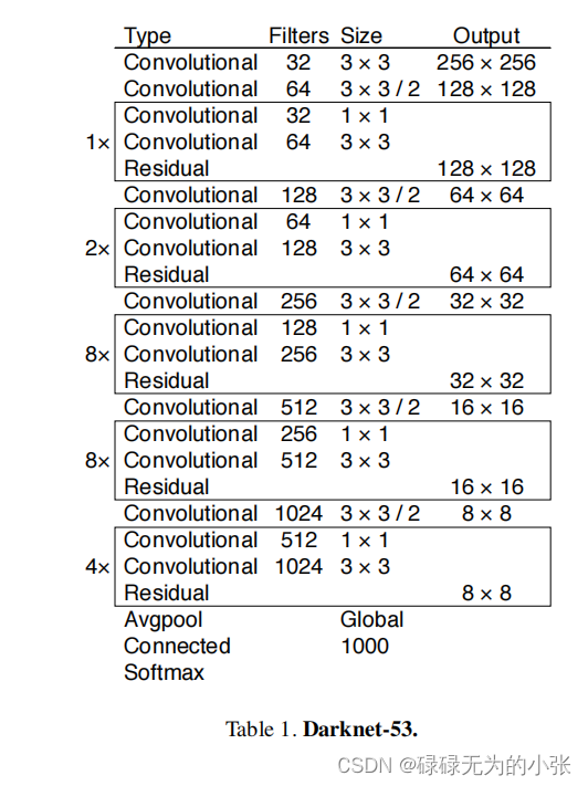
DarkNet的模型结构依旧采用了全卷积的方式，引入了残差连接的方式，增加的卷积的层数，模型结构变得更加复杂，整体而言跟DarkNet-19的变化不是很大。

先验框

相较于YOLOv2中5个先验框，作者使用了9个先验框，并将它们分为三个种类，分别是大中小三种。其中每一种对应三个先验框。所以在模型输出中输出了三种特征图，分别是$13\times 13$、$26\times 26$，$52\times 52$。这样对于不同大小的目标可以用不同的先验框进行匹配。同时，作者对它们做预测时不是直接采用Darknet输出的特征图，而是将尺度较小的特征图通过上采样的方式和特征图合并，然后进行预测，这种方式也可以认为是特征金字塔，可以加强对特征的提取。
作者在训练中对先验框的匹配规则跟之前的方式相似，每个真实标签只匹配一个与其最佳匹配的先验框，同时匹配的最小IOU应当大于0.5。

分类预测

作者不是使用softmax进行预测，而是使用logistic regression进行分类预测，即对一个类别预测一次，同时在训练时采用交叉损失熵的方式。所以每个预测头的输出大小为$(N\times N\times [3\ast (4+1+C)])$，这里$N$指特征图大小，3为该特征图对应的先验框数，4为预测的中心偏移和长宽缩扩比例，C为分类的数量。

整体而言，yolov3相较于yolov2没有太大的改变，更像是在原有基础上的一种延伸。