数据存储格式——SingleCellExperiment
https://osca.bioconductor.org/data-infrastructure.html
SingleCellExperiment - 简书 (jianshu.com)
为什么要以数据库的思维来理解单细胞数据 - 简书 (jianshu.com)
Bioconductor - Removed Packages
一、介绍
Bioconductor软件包SingleCellExperiment提供了SingleCellExperiment类以供使用。当使用依赖于SingleCellExperiment类的任何程序包和加载程序包时,可以按以下方式显式安装(并加载)程序包:
BiocManager::install('SingleCellExperiment')
BiocManager::install(c('scater', 'scran', 'uwot'))
library(SingleCellExperiment)
链接:https://www.jianshu.com/p/7dedf284ca54
二、数据结构
所述SingleCellExperiment(sce)对象是基于在Bioconductor的单细胞分析应用的基础。该sce对象是一个S4对象,与R中其他可用的方法相比,它本质上为数据的构造和访问提供了一种更为形式化的方法。
如果我们想象sce对象是一艘船,slots可被认为是个别货箱——为sce对象内单独的实体。此外,每个slot都包含自己的格式数据。打个比喻,我们可以想象水果和砖头需要不同的货箱变化形式。在某些情况下sce,一些slot包含矩阵,而其他slot则是数据框。
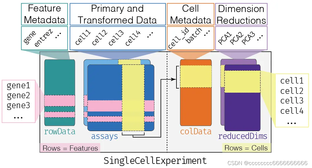
如上图所示,sce结构围绕scRNA-seq的原始count数据,储存了4组相关信息
- (1)Assays,即counts表达矩阵的标准化处理的矩阵(可以有任意多种,但常见的也就两三种);
- (2)colData,即scRNA-seq的每个细胞的信息(例如批次信息、分组信息、表达概况信息);
- (3)rowData,即scRNA-seq的每个基因的信息(例如表达概况、不同类基因名ID);
- (4)reducedDims,即每个细胞的降维特征信息(主要有PCA、tSNE、uMAP三类)
-
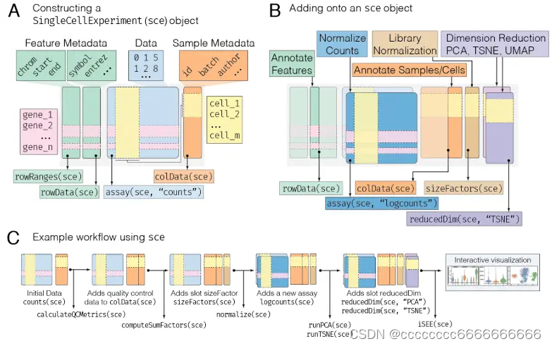
A : 最小的sce对象是通过提供数据来构建的,比如每个细胞的计数矩阵(蓝色方框),由特征组成,比如基因(行)和细胞(列)。还可以提供描述单元格的元数据,其中单元格表示为行,单元格的已知特征为列(橙色框)。类似地,也可以添加描述特性的元数据(绿色框)。这些不同类型的数据都存储在sce对象的不同部分中,这些部分称为槽(slots)。每个槽中的数据可以通过以各自的槽(箭头)命名的访问器以编程方式访问,比如rowRanges指的是特征元数据,colData指的是样本元数据,assay指的是数据。
-
B : 使用sce (singlecellexper, sce)兼容的工作流进行分析,将数据附加到初始sce对象。例如,计算每个单元格的库规范化因子将创建一个新槽(粉色框)。这些可以用来推导一个归一化计数矩阵,它与初始计数数据(深蓝色方框)一起存储在同一个检测槽中。因此,分析槽能够存储任意数量的数据转换。单元质量度量(描述单元特征)被附加到样例元数据槽colData中。最后,以与分析槽类似的方式,可以存储任意数量的维数缩减的数据表示形式,驻留在它们自己的槽中,reducedDim。
-
C : sce对象在典型分析的整个过程中不断发展,存储来自初始数据的各种度量和表示
三、R包准备与简单构建sce
1.安装
主要用到两个包:SingleCellExperiment,是构建sce对象的基础包;scater,是分析scRNA-seq的常用工具包之一。值得一提的是加载基于sce的单细胞分析工具包时都会自动加载包括SingleCellExperiment在内的依赖包。
BiocManager::install('SingleCellExperiment')
BiocManager::install('scater')
library(SingleCellExperiment)
library(scater)
2.简单构建sce
- 简单构建sce对象只需要提供单细胞count表达矩阵即可;
- 如下,模拟一个包含3个细胞,比对到10个基因上的count表达矩阵
counts_matrix <- data.frame(cell_1 = rpois(10, 10),
                            cell_2 = rpois(10, 10),
                            cell_3 = rpois(10, 30))
rownames(counts_matrix) <- paste0("gene_", 1:10)
counts_matrix <- as.matrix(counts_matrix) # must be a matrix object!
#           cell_1 cell_2 cell_3
# gene_1      17     12     21
# gene_2      14      6     36
# gene_3      12     11     30
# gene_4       8     15     26
# gene_5      15     11     31
# gene_6       9      8     29
# gene_7       8     12     28
# gene_8       7     10     32
# gene_9       9     10     27
# gene_10      6      6     26
sce <- SingleCellExperiment(assays = list(counts = counts_matrix))
sce
# class: SingleCellExperiment
# dim: 10 3
# metadata(0):
# assays(1): counts
#rownames(10): gene_1 gene_2 ... gene_9 gene_10
#rowData names(0):
#colnames(3): cell_1 cell_2 cell_3
#colData names(0):
#reducedDimNames(0):
#altExpNames(0):
四、sce四组成
1 .标准化数据之assays
相关函数命令
assays(sce)查看当前sce对象的所有assays' name【暂且可理解一种表达矩阵称之为一个assay】assay(sce,"name")查看sce指定一种assay的表达矩阵 针对常见的assay,例如count assay、logcounts assay。SingleCellExperiment包也提供了简单的查询方式,具体如下例。assay(sce,"new_name") = new_assay添加新的assay
assays(sce)
# List of length 1
# names(1): counts

#使用scater包标准化,可直接作用于sce对象;具体为先进行文库因子校正,再log2转换。
sce=logNormCounts(sce)
assays(sce)
# List of length 2
# names(2): counts logcounts
assay(sce,"logcounts")
# cell_1   cell_2   cell_3
# gene_1  4.784105 4.356506 3.705089
# gene_2  4.515174 3.425268 4.435852
# gene_3  4.303259 4.237364 4.186088
# gene_4  3.754379 4.664280 3.991779
# gene_5  4.610498 4.237364 4.230835
# gene_6  3.912376 3.806334 4.139909
# gene_7  3.754379 4.356506 4.092203
# gene_8  3.576925 4.107489 4.274236
# gene_9  3.912376 4.107489 4.042865
# gene_10 3.374543 3.425268 3.991779

counts(sce)
?counts
logcounts(sce)

#模拟一个新的assay
counts_100 <- counts(sce) + 100
assay(sce, "counts_100") <- counts_100 # assign a new entry to assays slot
assays(sce) # new assay has now been added.
2. 细胞信息之colData
主要包括两类:一是细胞的实验、分组等信息;二是根据表达矩阵概括的每个细胞的表达信息。
相关函数命令有colData(sce) 查看当前sce对象所有的细胞信息;配合美元符可方便的用于查看或新添某一条colData。尤其特殊一点是colData(sce)foo等价于sce
#当前sce有一条sizeFactor cell-info,为scater::logNormCounts时自动添加的
colData(sce)
# DataFrame with 3 rows and 1 column
# sizeFactor
# <numeric>
# cell_1   0.640244
# cell_2   0.615854
# cell_3   1.743902

#添加批次信息
#colData(sce)$batch
sce$batch=c(1,1,2)  #注意顺序要一致
colnames(colData(sce))
#[1] "batch"      "sizeFactor"

#也可在构建sce对象时,就添加上
cell_metadata <- data.frame(batch = c(1, 1, 2))
rownames(cell_metadata) <- paste0("cell_", 1:3)
sce <- SingleCellExperiment(assays = list(counts = counts_matrix),
                            colData = cell_metadata)

#利用scater包,注释每个细胞的表达概况
sce <- scater::addPerCellQC(sce)
colData(sce)
# DataFrame with 3 rows and 9 columns
# batch sizeFactor       sum  detected percent_top_50 percent_top_100 percent_top_200 percent_top_500     total
#           <numeric>  <numeric> <integer> <integer>      <numeric>       <numeric>       <numeric>       <numeric> <integer>
# cell_1         1   0.640244       105        10            100             100             100             100       105
# cell_2         1   0.615854       101        10            100             100             100             100       101
# cell_3         2   1.743902       286        10            100             100             100             100       286
3. gene信息之colData
我目前所认识主要包括两类:一是不同种基因ID,二是基因的表达情况
相关函数命令有 rowData(sce)
#利用scater包注释基因的表达情况
sce <- scater::addPerFeatureQC(sce)
rowData(sce)
# DataFrame with 10 rows and 2 columns
# mean  detected
# <numeric> <numeric>
# gene_1    16.6667       100
# gene_2    18.6667       100
# gene_3    17.6667       100
# gene_4    16.3333       100
# gene_5    19.0000       100
# gene_6    15.3333       100
# gene_7    16.0000       100
# gene_8    16.3333       100
# gene_9    15.3333       100
# gene_10   12.6667       100
4 .细胞降维信息之reducedDims
细胞降维信息,简单来说就是根据每个细胞的上千维表达情况压缩成几十个,甚至几个特征属性从而概括这个细胞的表达特征。方式有很多,常见的有三种PCA、tSNE、uMAP
相关函数有
reduceDims(sce)#查看当前sce有几种降维结果reduceDim(sce, "name")#查看具体某一种降维结果reduceDim(sce, "new_name") = foo#添加新一种降维结果,不过一个直接在sce对象中添加
reducedDims(sce)
# List of length 0
# names(0):

#利用scater包进行PCA降维
sce <- runPCA(sce)
reducedDims(sce)
# List of length 1
# names(1): PCA
reducedDim(sce, "PCA")
# PC1        PC2
# cell_1 -0.8716428822 -0.4312495
# cell_2  0.8713921135 -0.4316219
# cell_3  0.0002507686  0.8628713
# attr(,"percentVar")
# [1] 57.63049 42.36951
# attr(,"rotation")
# PC1         PC2
# gene_2  -0.62521538  0.35993511
# gene_1  -0.24546126 -0.66840778
# gene_4   0.52198543 -0.16823377
# gene_8   0.30446210  0.33370288
# gene_10  0.02919931  0.45728195
# gene_7   0.34545403  0.02830107
# gene_5  -0.21410318 -0.14912623
# gene_6  -0.06079117  0.21677758
# gene_9   0.11194401  0.02541130
# gene_3  -0.03781870 -0.06506096
五、sce取子集
- 如上,sce的四部分都是基于原始的细胞名和gene名搭建的。
- 如果只取其中一个细胞信息,则其余注释信息也当相应的取该细胞的注释信息;同理对基因筛选也是。
sce
# class: SingleCellExperiment
# dim: 10 3
# metadata(0):
# assays(2): counts logcounts
# rownames(10): gene_1 gene_2 ... gene_9 gene_10
# rowData names(2): mean detected
# colnames(3): cell_1 cell_2 cell_3
# colData names(10): batch sizeFactor ... total foo
# reducedDimNames(1): PCA
# altExpNames(0):

sce[1:2,]  #筛选基因
# class: SingleCellExperiment
# dim: 2 3
# metadata(0):
# assays(2): counts logcounts
# rownames(2): gene_1 gene_2
# rowData names(2): mean detected
# colnames(3): cell_1 cell_2 cell_3
# colData names(10): batch sizeFactor ... total foo
# reducedDimNames(1): PCA
# altExpNames(0):

sce[,c(1,3)]  #筛选细胞
sce[,sce$batch==1]  #根据注释信息筛选
六、简单对比Seurat数据结构
library(Seurat)
scRNA=as.Seurat(sce)
scRNA
# An object of class Seurat
# 10 features across 3 samples within 1 assay
# Active assay: RNA (10 features, 0 variable features)
#  1 dimensional reduction calculated: PCA
scRNA@assays$RNA@counts   #对应sce的counts assay
scRNA@assays$RNA@data     #对应sce的log2count assay
scRNA@meta.data           #对应sce的colData
scRNA@assays$RNA@meta.features  #应该对应sce的rowData,但显示为空值
scRNA@reductions$PCA@cell.embeddings #对应sce的reduceDim
subset(scRNA, subset = batch == 1)  #利用subset取子集

魔乐社区(Modelers.cn) 是一个中立、公益的人工智能社区,提供人工智能工具、模型、数据的托管、展示与应用协同服务,为人工智能开发及爱好者搭建开放的学习交流平台。社区通过理事会方式运作,由全产业链共同建设、共同运营、共同享有,推动国产AI生态繁荣发展。
更多推荐


 0
0 0
0- 0


 已为社区贡献5条内容

所有评论(0)