视觉SLAM十四讲学习4 (1)刚体变换与李群,李代数
视觉SLAM十四讲学习4 刚体变换与李群,李代数前言群定义李群与李代数的引出正交群与欧式群李代数的引出李代数so(3)so(3)so(3)的几何意义李群与李代数的转换后记前言本篇记录SLAM十四讲中的,李群与李代数。本篇与群论相关,因此相当不是很好理解。我反复看了五遍以上才稍微弄懂这一章。群定义群是一个集合GGG与一种运算◊\Diamond◊的复合,满足:1.封闭性:∀a,b∈G,a◊b∈G\fo
视觉SLAM十四讲学习4 刚体变换与李群,李代数
前言
本篇记录SLAM十四讲中的,李群与李代数。本篇与群论相关,因此相当不是很好理解。我反复看了五遍以上才稍微弄懂这一章。
群定义
群是一个集合 G G G与一种运算 ◊ \Diamond ◊的复合,满足:
1.封闭性: ∀ a , b ∈ G , a ◊ b ∈ G \forall a,b\in G, a\Diamond b\in G ∀a,b∈G,a◊b∈G
2.结合律: ∀ a , b ∈ G , a ◊ b = b ◊ a \forall a,b\in G, a\Diamond b=b\Diamond a ∀a,b∈G,a◊b=b◊a
3.幺元 ∃ e ∈ G , ∀ a ∈ G , a ◊ e = e ◊ a = a \exist e\in G,\forall a\in G, a\Diamond e=e\Diamond a=a ∃e∈G,∀a∈G,a◊e=e◊a=a
4.逆元: ∀ a ∈ G , ∃ b ∈ G , a ◊ b = b ◊ a = e \forall a\in G,\exist b \in G,a\Diamond b=b\Diamond a=e ∀a∈G,∃b∈G,a◊b=b◊a=e
比如实数集与加法组成一个群:
a + b ∈ R a + b + c = a + ( b + c ) a + 0 = 0 + a = a a + ( − a ) = 0 a+b \in R \\ a+b+c=a+(b+c) \\ a+0=0+a=a \\ a + (-a) =0 a+b∈Ra+b+c=a+(b+c)a+0=0+a=aa+(−a)=0
李群与李代数的引出
之前提到的刚体变换的矩阵表示方法,即旋转矩阵 R R R和变换矩阵 T T T,都存在参数冗余以及自约束的问题。因而需要引入更方便数值计算的方法。
所谓李群,是实数域上的具有连续性质的群,并且局部可导。下面着重介绍正交群 S O ( 3 ) SO(3) SO(3)与欧式群 S E ( 3 ) SE(3) SE(3)。
正交群与欧式群
特殊正交群记为 S O ( 3 ) = { R 3 × 3 ∣ R R T = I , d e t ( R ) = 1 } SO(3)=\{R_{3\times 3}|RR^T=I,det(R)=1 \} SO(3)={R3×3∣RRT=I,det(R)=1},可用于表示连续的三维旋转。
特殊欧式群记为 S E ( 3 ) = { T ∣ T = [ R t 0 1 ] , R ∈ S O ( 3 ) , t 3 × 1 } SE(3)=\{T|T=\begin{bmatrix}R & t \\ 0 & 1 \end{bmatrix},R\in SO(3),t_{3\times1}\} SE(3)={T∣T=[R0t1],R∈SO(3),t3×1},可用于表示三维空间中的欧式变换。
李代数的引出
假设当前的旋转 R R R是时间 t t t的函数 R ( t ) R(t) R(t),并且当 t = 0 t=0 t=0时, R ( 0 ) = I R(0)=I R(0)=I。现在需要求旋转的速度:
R ( t ) R ( t ) T = I R ˙ ( t ) R ( t ) T + R ( t ) R ˙ ( t ) T = 0 R ˙ ( t ) R ( t ) T = − R ( t ) R ˙ ( t ) T = − ( R ˙ ( t ) R ( t ) T ) T R(t)R(t)^T=I \\ \dot R(t)R(t)^T+R(t)\dot R(t)^T=0 \\ \dot R(t)R(t)^T = -R(t)\dot R(t)^T=-(\dot R(t)R(t)^T)^T R(t)R(t)T=IR˙(t)R(t)T+R(t)R˙(t)T=0R˙(t)R(t)T=−R(t)R˙(t)T=−(R˙(t)R(t)T)T
因为 R ˙ ( t ) R ( t ) T \dot R(t)R(t)^T R˙(t)R(t)T是一个反对称矩阵,因此可以找到一个向量 ϕ ( t ) \phi(t) ϕ(t),其反对称矩阵满足 ϕ ( t ) ∧ = R ˙ ( t ) R ( t ) T \phi(t)^\land=\dot R(t)R(t)^T ϕ(t)∧=R˙(t)R(t)T,有:
R ˙ ( t ) = ϕ ( t ) ∧ R ( t ) R ( 0 ) = I \dot R(t)=\phi(t)^\land R(t) \\ R(0)=I R˙(t)=ϕ(t)∧R(t)R(0)=I
上面的式子是一个带初值条件的矩阵微分方程,求解方法与普常微分方程类似:
R ( t ) = e ϕ ( t ) ∧ t R(t)=e^{\phi(t)^\land t} R(t)=eϕ(t)∧t
因此,任意时刻的旋转矩阵 R R R都与一个特定的向量 ϕ \phi ϕ的反对称矩阵具有指数映射的关系。 ϕ \phi ϕ就是 R R R对应的李代数 s o ( 3 ) so(3) so(3)。
李代数
对于不满足加运算的李群,不能直接通过李群求导,因此需要借助李代数来求导。
李代数是由一个集合、一个数域和一个二元运算李括号组成,李括号表示为: [ x , y ] [x,y] [x,y]。对于每个李群,都有对应的李代数,不同李代数的李括号并不相同。 s o ( 3 ) so(3) so(3)的李括号表示为:
[ ϕ 1 , ϕ 2 ] = ( ϕ 1 ∧ ϕ 2 ∧ , ϕ 2 ∧ ϕ 1 ∧ ) ∨ [\phi_1,\phi_2]=(\phi_1^\land\phi_2^\land,\phi_2^\land\phi_1^\land)^\lor [ϕ1,ϕ2]=(ϕ1∧ϕ2∧,ϕ2∧ϕ1∧)∨
s o ( 3 ) = { ϕ ∈ R 3 , ϕ ∧ ∈ R 3 × 3 } so(3)=\{\phi \in {\bf R^3},\phi ^\land\in {\bf R^{3\times 3}} \} so(3)={ϕ∈R3,ϕ∧∈R3×3}
s o ( 3 ) so(3) so(3)的几何意义
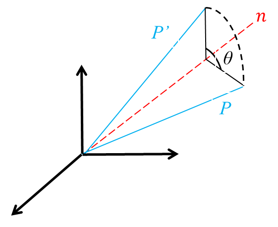
如上图所示是一个向量 P P P绕着单位向量 n n n旋转 θ \theta θ角度后得到 P ′ P' P′。假设 t = 0 t=0 t=0时, P ( 0 ) = P P(0)=P P(0)=P,绕 n n n旋转的角速度为1rad/s,则t时刻的向量位置可表示为 P ( t ) P(t) P(t),并且 P ( θ ) = P ′ P(\theta)=P' P(θ)=P′。 P ( t ) P(t) P(t)的瞬时速度 P ′ ( t ) P'(t) P′(t)是 P P P绕 n n n的线速度:
P ′ ( t ) = n × P ( t ) P ˙ ( t ) = n ∧ P ( t ) P'(t)=n\times P(t) \\ \dot P(t)=n^\land P(t) P′(t)=n×P(t)P˙(t)=n∧P(t)
这与上面李代数与旋转 R R R的映射表达式相同。
李群与李代数的转换
已知 S O ( 3 ) SO(3) SO(3)与 s o ( 3 ) so(3) so(3)之间的映射为 R = e ϕ ∧ t R=e^{\phi^\land t} R=eϕ∧t,现在需要进行 s o ( 3 ) 与 S O ( 3 ) so(3)与SO(3) so(3)与SO(3)之间的转换:
e ϕ ∧ t = I + ϕ ∧ + 1 2 ( ϕ ∧ ) 2 + 1 3 ! ( ϕ ∧ ) 3 + 1 4 ! ( ϕ ∧ ) 4 + … e^{\phi^\land t}=I+\phi^\land +\frac{1}{2}(\phi^\land)^2+\frac{1}{3!}(\phi^\land)^3+\frac{1}{4!}(\phi^\land)^4+\dots eϕ∧t=I+ϕ∧+21(ϕ∧)2+3!1(ϕ∧)3+4!1(ϕ∧)4+…
对于以上展开式,需要通过 ϕ ∧ \phi^\land ϕ∧的化简进行:
ϕ = θ n , ∣ ∣ n ∣ ∣ 2 = 1 ϕ ∧ = θ n ∧ n ∧ n ∧ = n n T − I n ∧ n ∧ n ∧ = − n ∧ \phi = \theta n,||n||_2=1 \\ \phi^\land=\theta n^\land \\ n^\land n^\land=nn^T-I\\ n^\land n^\land n^\land=-n^\land ϕ=θn,∣∣n∣∣2=1ϕ∧=θn∧n∧n∧=nnT−In∧n∧n∧=−n∧
代回展开式:
e ϕ ∧ t = n n T − n ∧ n ∧ + θ n ∧ + θ 2 2 ! ( n n T − I ) + θ 3 3 ! ( − n ∧ ) + … = n n T + ( θ − θ 3 3 ! + θ 5 5 ! + … ) n ∧ − ( 1 − θ 2 2 ! + θ 4 4 ! + … ) n ∧ n ∧ = n n T + n ∧ sin θ − n ∧ n ∧ cos θ = n n T + n ∧ sin θ − n n T cos θ + I cos θ = n n T ( 1 − cos θ ) + n ∧ sin θ + I cos θ e^{\phi^\land t}=nn^T-n^\land n^\land+\theta n^\land +\frac{\theta^2}{2!}(nn^T-I)+\frac{\theta^3}{3!}(-n^\land) + \dots \\ =nn^T+ (\theta -\frac{\theta^3}{3!}+\frac{\theta^5}{5!}+\dots)n^\land -(1-\frac{\theta^2}{2!}+\frac{\theta^4}{4!}+\dots)n^\land n^\land \\ = nn^T +n^\land \sin\theta - n^\land n^\land \cos \theta \\ = nn^T + n^\land \sin \theta - nn^T\cos \theta +I\cos \theta \\ = nn^T(1-\cos\theta) +n^\land \sin \theta + I\cos \theta\\ eϕ∧t=nnT−n∧n∧+θn∧+2!θ2(nnT−I)+3!θ3(−n∧)+…=nnT+(θ−3!θ3+5!θ5+…)n∧−(1−2!θ2+4!θ4+…)n∧n∧=nnT+n∧sinθ−n∧n∧cosθ=nnT+n∧sinθ−nnTcosθ+Icosθ=nnT(1−cosθ)+n∧sinθ+Icosθ
实际上就是刚体变换中的罗德里格斯公式。这也表明了 s o ( 3 ) so(3) so(3)与 S O ( 3 ) SO(3) SO(3)的关系,就是旋转矩阵与旋转向量之间的关系。
后记
由于李群这章比较长,因此下次再记录李群求导的方法。

魔乐社区(Modelers.cn) 是一个中立、公益的人工智能社区,提供人工智能工具、模型、数据的托管、展示与应用协同服务,为人工智能开发及爱好者搭建开放的学习交流平台。社区通过理事会方式运作,由全产业链共同建设、共同运营、共同享有,推动国产AI生态繁荣发展。
更多推荐


 0
0 0
0- 0


 已为社区贡献4条内容

所有评论(0)