异常检测

1、可视化数据

def visualize_dataset(X):
    plt.scatter(X[..., 0], X[..., 1], marker="x", label="point")

2、估计参数

def estimate_parameters_for_gaussian_distribution(X):
    mu = np.mean(X, axis=0)
    sigma2 = np.var(X, axis=0)
    return mu, sigma2

3、根据高斯模型，计算概率

def gaussian_distribution(X, mu, sigma2):
    p = np.exp(-(X-mu)**2/(2*sigma2)) * 1/(np.sqrt(2*np.pi*sigma2))
    return np.prod(p, axis=1)

4、画出高斯分布的等高线

def visualize_contours(mu, sigma2):
    x, y = np.linspace(5, 25, 100), np.linspace(5, 25, 100)
    xx, yy = np.meshgrid(x, y)
    X = np.concatenate((xx.reshape(-1, 1), yy.reshape(-1, 1)), axis=1)
    z = gaussian_distribution(X, mu, sigma2).reshape(xx.shape)
    cont_levels = [10**h for h in range(-20, 0, 3)]  # 当z为当前列表的值时才绘出等高线
    plt.contour(xx, yy, z, cont_levels)

5、计算precision、recall

# yp是预测值，yt是真实值  
def error_analysis(yp, yt):
    tp, fp, fn, tn = 0, 0, 0, 0
    for i in range(len(yp)):
        if yp[i] == yt[i]:
            if yp[i] == 1:
                tp += 1
            else:
                tn += 1
        else:
            if yp[i] == 1:
                fp += 1
            else:
                fn += 1
    precision = tp / (tp+fp) if tp + fp else 0
    recall = tp / (tp+fn) if tp+fn else 0
    f1 = 2*precision*recall/(precision+recall) if precision+recall else 0
    return f1

6、选择最好的阈值

# yval真实值 pval预测值
def select_threshold(yval, pval):
    epsilons = np.linspace(min(pval), max(pval), 1000)
    l = np.zeros((1, 2))
    for e in epsilons:
        ypre = (pval<e).astype(float)
        f1 = error_analysis(ypre, yval)
        l = np.concatenate((l, np.array([[e, f1]])), axis=0)
    index = np.argmax(l[..., 1])
    return l[index, 0], l[index, 1]

7、根据高斯模型检测出异常数据

def detection(X, e, mu, sigma2):
    p = gaussian_distribution(X, mu, sigma2)
    anomaly_points = np.array([X[i] for i in range(len(p)) if p[i]<e])
    return anomaly_points

8、可视化异常数据

def circle_anomaly_points(X):
    plt.scatter(X[..., 0], X[..., 1], s=80, facecolor="none", edgecolors="r", label="anomaly point")

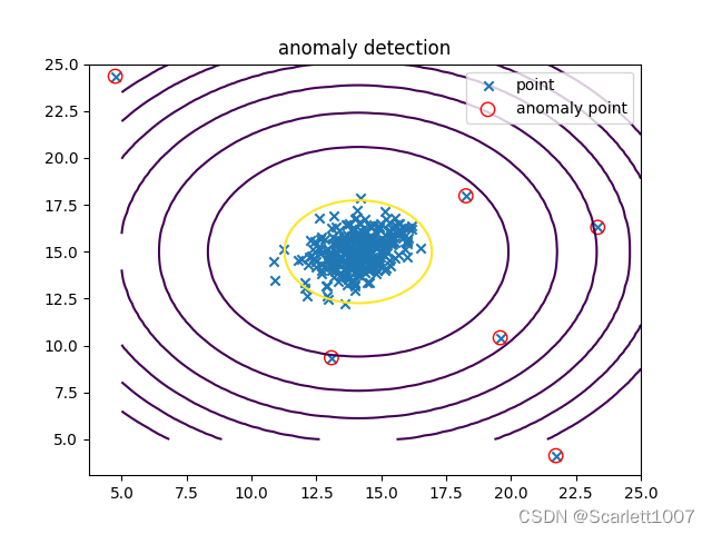
9、低维数据测试

data = sio.loadmat(文件路径)
    X = data["X"]  # (307,2)
    visualize_dataset(X)
    mu, sigma2 = estimate_parameters_for_gaussian_distribution(X)  # [14.11222578 14.99771051] [1.83263141 1.70974533]
    p = gaussian_distribution(X, mu, sigma2)  # (307,)
    visualize_contours(mu, sigma2)

    Xval = data["Xval"]  # (307,2)
    yval = data["yval"]  # (307,1)
    print(yval[:3])
    e, f1 = select_threshold(yval.ravel(), gaussian_distribution(Xval, mu, sigma2))
    print('best choice of epsilon is ', e, ',the F1 score is ', f1)
    # best choice of epsilon is  8.999852631901394e-05 ,the F1 score is  0.8750000000000001
    anomaly_points = detection(X, e, mu, sigma2)
    circle_anomaly_points(anomaly_points)
    plt.title('anomaly detection')
    plt.legend()
    plt.show()

10、高维数据测试

data2 = sio.loadmat(文件路径)
    X = data2["X"]  # (1000,11)
    Xval = data2["Xval"]  # (100,11)
    yval = data2["yval"]  # (100, 1)
    mu, sigma2 = estimate_parameters_for_gaussian_distribution(X)
    e, f1 = select_threshold(yval.ravel(), gaussian_distribution(Xval, mu, sigma2))
    anomaly_points = detection(X, e, mu, sigma2)
    print('\n\nfor this high dimensional dataset \nbest choice of epsilon is ', e, ',the F1 score is ', f1)
    print('the number of anomaly points is', anomaly_points.shape[0])
    # for this high dimensional dataset 
    # best choice of epsilon is  1.3786074982000235e-18 ,the F1 score is  0.6153846153846154
    # the number of anomaly points is 117

 

推荐系统

1、导入所需的库

import scipy.io as sio
import numpy as np
import scipy.optimize as opt
from sklearn.metrics import mean_squared_error

2、参数维数变换

# 参数一维向量化
def serialize(X, theta):
    return np.concatenate((X.flatten(), theta.flatten()), axis=0)


# 将一维参数向量还原
def deserializer(params, nm, nu, nf):
    X = params[: nm*nf].reshape(nm, nf)
    theta = params[nm*nf:].reshape(nu, nf)
    return X, theta

3、协同过滤算法目标函数

def collaborative_filtering_cost(params, Y, R, nm, nu, nf, lamda=0.0):
    X, theta = deserializer(params, nm, nu, nf)
    part1 = np.sum(((X.dot(theta.T) - Y) ** 2)*R)/2
    part2 = (lamda/2) * np.sum(theta**2)
    part3 = (lamda/2) * np.sum(X**2)
    return part1 +part2 + part3

4、协同过滤梯度下降

def collaborative_filtering_gradient(params, Y, R, nm, nu, nf, lamda=0.0):
    X, theta = deserializer(params, nm, nu, nf)
    g_X = ((X.dot(theta.T)-Y) * R).dot(theta) + lamda*X
    g_theta = ((X.dot(theta.T)-Y) * R).T.dot(X) + lamda*theta
    return serialize(g_X, g_theta)

5、检验预测

def check_gradient(params, Y, R, nm, nu, nf):
    e = 0.0001
    m = len(params)
    g_params = np.zeros((m,))
    for i in range(m):
        temp = np.zeros((m,))
        temp[i] = e
        g_params = (collaborative_filtering_cost(params+temp, Y, R, nm, nu, nf)-
                    collaborative_filtering_gradient(params-temp, Y, R, nm, nu, nf))/(2 * e)
    return g_params

6、代入数据

data1 = sio.loadmat(文件路径)
    # Y是包含从1到5的等级的（数量的电影x数量的用户）数组.R是包含指示用户是否给电影评分的二进制值的“指示符”数组。 两者应该具有相同的维度。
    Y = data1["Y"]  # (1682,943)
    R = data1["R"]  # (1682,943)
    data2 = sio.loadmat(r"E:\zl\机器学习\1\data\ex8\ex8_anomaly_detection_and_recommender_system_data_ex8_movieParams")
    X = data2["X"]  # (1682,10)
    theta = data2["Theta"]  # (943,10)
    nu = data2["num_users"][0][0]  # 943
    nm = data2["num_movies"][0][0]  # 1682
    nf = data2["num_features"][0][0]  # 10
    print(collaborative_filtering_cost(serialize(X, theta), Y, R, nm, nu, nf))  # 27918.64012454421
    print(collaborative_filtering_cost(serialize(X, theta), Y, R, nm, nu, nf, 1.5))  # 34821.703613072226

# 读入电影标签
    with open(文件路径) as f:
        movies = []
        for line in f.readlines():
            movies.append(line.split(' ', 1)[-1])

    # 训练模型
    # 添加一组自定义的用户数据
    my_ratings = np.zeros((1682, 1))
    my_ratings[0] = 4
    my_ratings[97] = 2
    my_ratings[6] = 3
    my_ratings[11] = 5
    my_ratings[53] = 4
    my_ratings[63] = 5
    my_ratings[65] = 3
    my_ratings[68] = 5
    my_ratings[182] = 4
    my_ratings[225] = 5
    my_ratings[354] = 5
    Y = np.concatenate((Y, my_ratings), axis=1)
    R = np.concatenate((R, my_ratings > 0), axis=1)
    nu += 1
    # params = serialize(np.random.random((nm, nf)), np.random.random((nu, nf)))
    # res = opt.minimize(fun=collaborative_filtering_cost, x0=params, args=(Y, R, nm, nu, nf,10), method="TNC",
    #                    jac=collaborative_filtering_gradient)
    # print(res.shape)
    trained_X, trained_theta = deserializer(sio.loadmat(文件路径)["params"].ravel(), nm, nu, nf)
    predict = trained_X.dot(trained_theta.T)
    my_predict = predict[..., -1]

    # 从预测结果选择10个最优推荐
    for i in range(10):
        index = int(np.argmax(my_predict))
        print("Predicting rating ", my_predict[index], " for movie ", movies[index])
        my_predict[index] = -1
    # Predicting
    # rating
    # 4.291401160077979
    # for movie  Titanic(1997)
    #
    # Predicting
    # rating
    # 4.119953862808096
    # for movie  Star Wars (1977)
    #
    # Predicting
    # rating
    # 3.9792200003762264
    # for movie  Raiders of the Lost Ark (1981)
    #
    # Predicting
    # rating
    # 3.9099976364851314
    # for movie  Good Will Hunting (1997)
    #
    # Predicting
    # rating
    # 3.885805506896392
    # for movie  Shawshank Redemption, The (1994)
    #
    # Predicting
    # rating
    # 3.8729551652292584
    # for movie  Return of the Jedi (1983)
    #
    # Predicting
    # rating
    # 3.8712945387591366
    # for movie  Braveheart(1995)
    #
    # Predicting
    # rating
    # 3.863004536777663
    # for movie  Empire Strikes Back, The (1980)
    #
    # Predicting
    # rating
    # 3.757933676945382
    # for movie  Terminator 2: Judgment
    # Day(1991)
    #
    # Predicting
    # rating
    # 3.7576861972110667
    # for movie  As Good As It Gets (1997)

    # 用均方误差来评价
    Y = Y.flatten()
    R = R.flatten()
    predict = predict.flatten()
    true_y = []
    pre_y = []
    for i in range(len(Y)):
        if R[i] == 1:
            true_y.append(Y[i])
            pre_y.append(predict[i])
    print("当前训练对岳原始数据集的均方误差", mean_squared_error(true_y, pre_y))  # 当前训练对岳原始数据集的均方误差 0.6400023155268085